Testing Robustness of SPD Models with Riemannian PGD Attack

This example demonstrates how to implement and evaluate the Riemannian Projected Gradient Descent (R-PGD) attack [Timoz et al., 2026] on models that operate on Symmetric Positive Definite (SPD) matrices using SPD Learn.

Citation

If you use this tutorial or the R-PGD attack implementation in your research, please cite:

Timoz, D., de Surrel, T., & Yger, F. (2026). Riemannian adversarial attacks
on Symmetric Positive Definite matrices. In International Conference on
Acoustics, Speech, and Signal Processing (ICASSP).

BibTeX entry:

@inproceedings{timoz2026riemannian,
  title={Riemannian adversarial attacks on Symmetric Positive Definite matrices},
  author={Timoz, D. and de Surrel, T. and Yger, F.},
  booktitle={International Conference on Acoustics, Speech, and Signal
             Processing - ICASSP},
  year={2026},
  pages={1--8},
  organization={Springer},
}

And please cite SPD Learn:

@article{aristimunha2025spdlearn,
  title={SPDlearn: A Geometric Deep Learning Python Library for
         Neural Decoding Through Trivialization},
  author={Aristimunha, Bruno and Ju, Ce and Collas, Antoine and
          Bouchard, Florent and Mian, Ammar and Thirion, Bertrand and
          Chevallier, Sylvain and Kobler, Reinmar},
  journal={To be submitted},
  year={2026},
  url={https://github.com/spdlearn/spd_learn}
}

Introduction

Deep neural networks are vulnerable to adversarial attacks due to their high capacity and sensitivity to small, carefully crafted perturbations. These vulnerabilities can be especially concerning when the models operate on geometrically structured inputs like SPD matrices, where preserving the intrinsic properties of the data is crucial.

The objective is to construct a perturbation of a SPD matrix such that the Riemannian distance to the original sample is minimal, while the prediction is completely altered (misclassified).

There are two main types of attacks:

• Black-box attacks: model parameters unknown, but predictions obtainable

• White-box attacks: model parameters known, gradients computable

Since a model robust to white-box attacks is generally robust to black-box attacks, we focus on white-box attacks.

For background on SPD geometry, see Geometry Essentials.

The R-PGD Attack Algorithm

One method behind adversarial attacks is to increase the loss function while respecting a budget constraint \(\epsilon\). The standard Projected Gradient Descent (PGD) attack performs gradient ascent with projections back onto a constraint ball.

However, Euclidean PGD fails on SPD matrices because:

1. Perturbations may leave the SPD manifold

2. The Euclidean distance doesn’t capture the intrinsic geometry

SPD Learn implements the Riemannian PGD attack that performs updates along the affine-invariant geometry:

\[\Sigma_{k+1} = \Pi_{B_\epsilon(\Sigma_0)} \left( \exp_{\Sigma_k}(\alpha \cdot \text{grad } J(\Sigma_k, Y)) \right)\]

where:

• \(\exp_{\Sigma}\) is the exponential map ensuring we stay on the manifold

• \(\Pi_{B_\epsilon}\) projects onto the geodesic ball of radius \(\epsilon\)

• \(\text{grad } J\) is the Riemannian gradient of the loss

The projection onto the ball \(B_\epsilon(\Sigma_0) = \{\Sigma \in S^d_{++} | \delta_r(\Sigma_0, \Sigma) \leq \epsilon\}\) uses:

\[\begin{split}\Pi_{B_\epsilon(\Sigma_0)}(\Sigma) = \begin{cases} \exp_{\Sigma_0}\left(\frac{\epsilon}{\delta_r(\Sigma_0,\Sigma)} \log_{\Sigma_0}(\Sigma)\right) & \text{if } \delta_r(\Sigma_0, \Sigma) > \epsilon \\ \Sigma & \text{otherwise} \end{cases}\end{split}\]

This ensures the attack respects the budget using Riemannian distance, which limits the loss of geometric information and helps preserve the semantics of the original sample.

Setup and Imports

import warnings

import matplotlib.pyplot as plt
import torch

from braindecode import EEGClassifier
from moabb.datasets import BNCI2014_001
from moabb.paradigms import MotorImagery
from sklearn.metrics import accuracy_score
from sklearn.preprocessing import LabelEncoder
from skorch.callbacks import EpochScoring, GradientNormClipping
from skorch.dataset import ValidSplit

from spd_learn.functional import spd_rpgd_attack
from spd_learn.models import SPDNet
from spd_learn.modules import CovLayer


warnings.filterwarnings("ignore")

/opt/hostedtoolcache/Python/3.11.16/x64/lib/python3.11/site-packages/braindecode/models/eegpt.py:497: FutureWarning: Montage name 'standard_1020' is deprecated and will be removed in MNE 1.14. Use 'colin27_1020' instead.
  montage = mne.channels.make_standard_montage("standard_1020")
/opt/hostedtoolcache/Python/3.11.16/x64/lib/python3.11/site-packages/braindecode/models/eegpt.py:1452: FutureWarning: Montage name 'standard_1020' is deprecated and will be removed in MNE 1.14. Use 'colin27_1020' instead.
  montage = make_standard_montage("standard_1020")

Data Preparation

We use the motor imagery dataset BNCI2014-001 from MOABB. Following the paper, we apply a band-pass filter with range [7; 35] Hz. We use a single subject for demonstration purposes.

subject_id = 1

dataset = BNCI2014_001()
paradigm = MotorImagery(n_classes=4, fmin=7, fmax=35)

# Prepare data
cov_layer = CovLayer()
X, labels, meta = paradigm.get_data(dataset=dataset, subjects=[subject_id])
X = torch.tensor(X, dtype=torch.float32)
X = cov_layer(X)
le = LabelEncoder()
y = le.fit_transform(labels)

# Split by session (inter-session setup as from the paper)
train_idx = meta.query("session == '0train'").index.to_numpy()
test_idx = meta.query("session == '1test'").index.to_numpy()

print(f"Training samples: {len(train_idx)}, Test samples: {len(test_idx)}")
print(f"SPD matrix shape: {X.shape[1]}x{X.shape[2]}")

Choosing from all possible events
Training samples: 288, Test samples: 288
SPD matrix shape: 22x22

Training the SPDNet Model

SPDNet [Huang and Van Gool, 2017] is a neural network architecture designed to operate on SPD matrices. It introduces three layers that preserve the intrinsic geometry:

• BiMap: bilinear projection \(f(\\Sigma) = W\\Sigma W^{\\top}\)

• ReEig: enforces positive eigenvalues via spectral rectification

• LogEig: maps to tangent space for Euclidean classification

The model contains 2 BiMap and ReEig layers followed by LogEig and FC layers.

n_chans = 22
model = SPDNet(input_type="cov", n_chans=n_chans, n_outputs=4)
clf = EEGClassifier(
    model,
    criterion=torch.nn.CrossEntropyLoss,
    optimizer=torch.optim.Adam,
    optimizer__lr=1e-3,
    train_split=ValidSplit(0.1, stratified=True, random_state=42),
    batch_size=32,
    max_epochs=20,
    callbacks=[
        (
            "train_acc",
            EpochScoring(
                "accuracy", lower_is_better=False, on_train=True, name="train_acc"
            ),
        ),
        ("gradient_clip", GradientNormClipping(gradient_clip_value=1.0)),
    ],
    verbose=1,
)

# Train
clf.fit(X[train_idx], y[train_idx])

  epoch    train_acc    train_loss    valid_acc    valid_loss     dur
-------  -----------  ------------  -----------  ------------  ------
      1       0.2070        1.4194       0.2759        1.3716  0.0754
      2       0.3438        1.3502       0.4138        1.3288  0.0711
      3       0.4141        1.3076       0.4483        1.2869  0.0669
      4       0.5391        1.2624       0.4483        1.2424  0.0714
      5       0.4688        1.2368       0.4828        1.2123  0.0695
      6       0.5898        1.1901       0.4828        1.1755  0.0706
      7       0.6758        1.1520       0.6207        1.1414  0.0677
      8       0.7305        1.1181       0.6207        1.1194  0.0709
      9       0.6133        1.0918       0.5517        1.0901  0.0696
     10       0.5781        1.0696       0.5517        1.0625  0.0723
     11       0.7539        1.0411       0.6897        1.0547  0.0672
     12       0.7539        1.0197       0.6552        1.0253  0.0707
     13       0.6836        1.0030       0.6552        1.0087  0.0673
     14       0.6680        0.9831       0.5517        0.9885  0.0699
     15       0.6953        0.9616       0.6897        0.9766  0.0702
     16       0.8125        0.9436       0.6207        0.9646  0.0695
     17       0.7383        0.9287       0.5517        0.9522  0.0708
     18       0.7969        0.9151       0.7241        0.9425  0.0699
     19       0.7695        0.9046       0.6552        0.9206  0.0685
     20       0.7266        0.8889       0.5517        0.9184  0.0717

<class 'braindecode.classifier.EEGClassifier'>[initialized](
  module_=SPDNet(
    (cov): Identity()
    (bimap): ParametrizedBiMap(
      (parametrizations): ModuleDict(
        (weight): ParametrizationList(
          (0): _Orthogonal()
        )
      )
    )
    (reeig): ReEig()
    (logeig): LogEig()
    (classifier): Linear(in_features=253, out_features=4, bias=True)
  ),
)

In a Jupyter environment, please rerun this cell to show the HTML representation or trust the notebook.
On GitHub, the HTML representation is unable to render, please try loading this page with nbviewer.org.

Implementing the Riemannian PGD Attack

We now use SPD Learn’s spd_rpgd_attack() to generate adversarial examples. The attack parameters are:

• eps: Maximum perturbation radius (geodesic budget)

• n_iterations: Number of PGD iterations (paper uses 50)

• step_size: Step size \(\alpha\) for each iteration (paper uses 0.1)

Following the paper, convergence is reached when the loss variation falls below \(10^{-4}\).

criterion = torch.nn.CrossEntropyLoss()

# Select samples to attack
X_test = X[test_idx]
y_test = y[test_idx]

initial_accuracy = accuracy_score(y_test, clf.predict(X_test))
print(f"Initial accuracy on clean test data: {initial_accuracy * 100:.2f}%")

# Parameters for the attack (from the paper)
epsilon = 0.5  # Maximum perturbation radius (geodesic budget)
n_iterations = 50  # Number of PGD iterations
step_size = 0.1  # Step size for each iteration (alpha in the paper)

# Generate adversarial examples
X_adv = spd_rpgd_attack(
    clf,
    X_test,
    torch.tensor(y_test),
    eps=epsilon,
    criterion=criterion,
    n_iterations=n_iterations,
    step_size=step_size,
)

# Evaluate the model on adversarial examples
adv_accuracy = accuracy_score(y_test, clf.predict(X_adv))
print(f"Accuracy on adversarial test data: {adv_accuracy * 100:.2f}%")
print(f"Attack success rate: {(1 - adv_accuracy / initial_accuracy) * 100:.2f}%")

Initial accuracy on clean test data: 66.32%
Accuracy on adversarial test data: 26.04%
Attack success rate: 60.73%

Evaluating Model Robustness Across Budgets

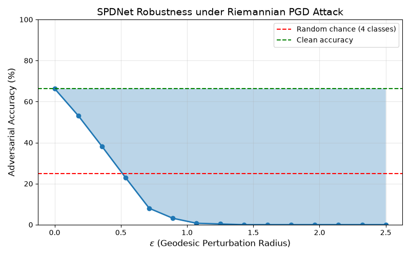
We evaluate the model’s robustness by attacking with different perturbation budgets. As shown in the paper, R-PGD keeps progressing steadily until it reaches 100% success rate, unlike Euclidean PGD which saturates.

This is because Euclidean attacks must follow curved trajectories on the manifold using straight-line updates. The frequent projections back onto the manifold decrease the effectiveness of each update.

epsilons = torch.linspace(0.0, 2.5, steps=15)
accuracies = []

for eps in epsilons:
    X_adv = spd_rpgd_attack(
        clf,
        X_test,
        torch.tensor(y_test),
        eps=eps.item(),
        criterion=criterion,
        n_iterations=n_iterations,
        step_size=step_size,
    )
    adv_accuracy = accuracy_score(y_test, clf.predict(X_adv))
    accuracies.append(adv_accuracy)
    print(f"Epsilon: {eps.item():.2f}, Adversarial Accuracy: {adv_accuracy * 100:.2f}%")

Epsilon: 0.00, Adversarial Accuracy: 66.32%
Epsilon: 0.18, Adversarial Accuracy: 53.12%
Epsilon: 0.36, Adversarial Accuracy: 38.19%
Epsilon: 0.54, Adversarial Accuracy: 22.92%
Epsilon: 0.71, Adversarial Accuracy: 7.99%
Epsilon: 0.89, Adversarial Accuracy: 3.12%
Epsilon: 1.07, Adversarial Accuracy: 0.69%
Epsilon: 1.25, Adversarial Accuracy: 0.35%
Epsilon: 1.43, Adversarial Accuracy: 0.00%
Epsilon: 1.61, Adversarial Accuracy: 0.00%
Epsilon: 1.79, Adversarial Accuracy: 0.00%
Epsilon: 1.96, Adversarial Accuracy: 0.00%
Epsilon: 2.14, Adversarial Accuracy: 0.00%
Epsilon: 2.32, Adversarial Accuracy: 0.00%
Epsilon: 2.50, Adversarial Accuracy: 0.00%

Visualizing the Results

We plot the adversarial accuracy as a function of the perturbation budget. The Riemannian distance can differ significantly from the Euclidean one and better captures the intrinsic geometry of the manifold, making it more appropriate in the context of adversarial attacks.

fig, ax = plt.subplots(figsize=(8, 5))
ax.plot(epsilons.numpy(), [acc * 100 for acc in accuracies], marker="o", linewidth=2)
ax.axhline(y=25, color="r", linestyle="--", label="Random chance (4 classes)")
ax.axhline(y=initial_accuracy * 100, color="g", linestyle="--", label="Clean accuracy")
ax.fill_between(
    epsilons.numpy(),
    [acc * 100 for acc in accuracies],
    initial_accuracy * 100,
    alpha=0.3,
)
ax.set_title("SPDNet Robustness under Riemannian PGD Attack", fontsize=14)
ax.set_xlabel(r"$\epsilon$ (Geodesic Perturbation Radius)", fontsize=12)
ax.set_ylabel("Adversarial Accuracy (%)", fontsize=12)
ax.legend(loc="upper right")
ax.grid(True, alpha=0.3)
ax.set_ylim(0, 100)
plt.tight_layout()
plt.show()

Comparing Clean vs Adversarial Predictions

We can visualize how predictions change under adversarial perturbations.

clean_preds = clf.predict(X_test)
adv_preds = clf.predict(X_adv)

# Count prediction changes
changed_mask = clean_preds != adv_preds
n_changed = changed_mask.sum()
n_total = len(y_test)

print(f"\nPrediction changes under attack (epsilon={epsilon}):")
print(
    f"  Changed predictions: {n_changed}/{n_total} ({100 * n_changed / n_total:.1f}%)"
)

# Confusion between clean and adversarial
fig, axes = plt.subplots(1, 2, figsize=(12, 5))

# Clean predictions
from sklearn.metrics import ConfusionMatrixDisplay


ConfusionMatrixDisplay.from_predictions(
    y_test, clean_preds, ax=axes[0], cmap="Blues", colorbar=False
)
axes[0].set_title(f"Clean Predictions\n(Accuracy: {initial_accuracy * 100:.1f}%)")

# Adversarial predictions
ConfusionMatrixDisplay.from_predictions(
    y_test, adv_preds, ax=axes[1], cmap="Oranges", colorbar=False
)
axes[1].set_title(f"Adversarial Predictions\n(Accuracy: {adv_accuracy * 100:.1f}%)")

plt.tight_layout()
plt.show()

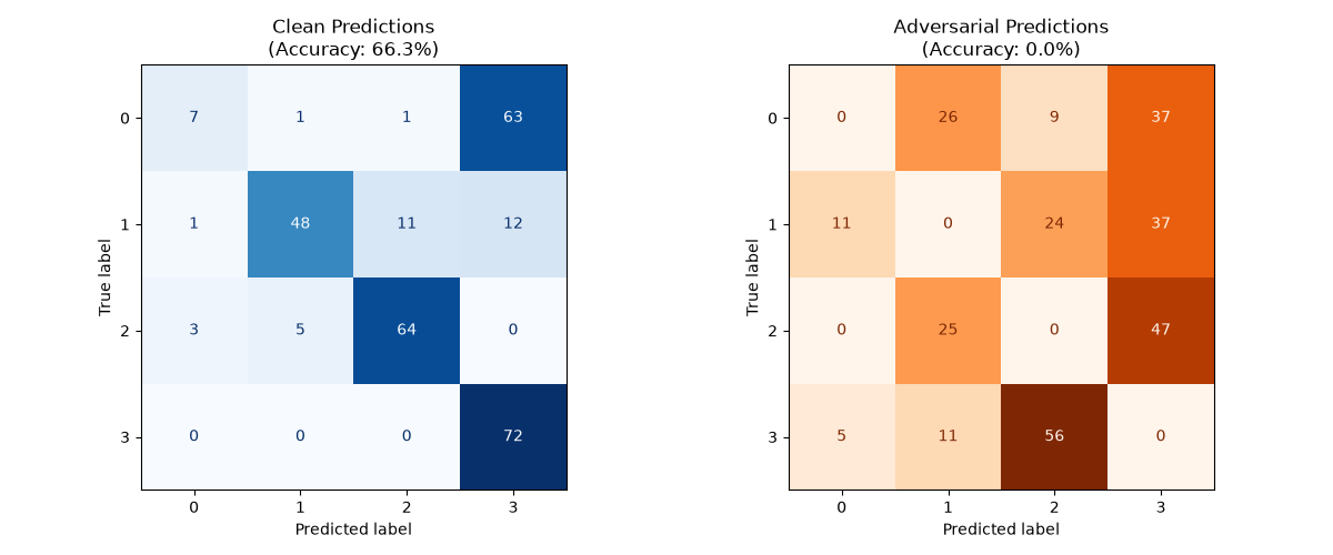
Prediction changes under attack (epsilon=0.5):
  Changed predictions: 226/288 (78.5%)

Why Riemannian Attacks Outperform Euclidean Attacks

The paper demonstrates that Euclidean PGD encounters increasing difficulty in completely degrading the model’s performance beyond a certain budget. This happens because:

1. At higher budgets, Euclidean attacks tend to move outside the SPD manifold

2. The mandatory projection step significantly reduces effective perturbation

3. Euclidean attacks approximate curved geodesics with straight-line updates

In contrast, R-PGD:

• Stays on the manifold by construction (using exponential map)

• Respects the intrinsic geometry with Riemannian gradients

• Uses geodesic distance for meaningful budget constraints

The Riemannian PGD attack has the advantage of defining the attack budget using a Riemannian distance, which limits the loss of geometric information caused by the attack and helps preserve the semantics of the original sample.

Conclusion

In this example, we demonstrated how to use SPD Learn to implement the Riemannian PGD attack on SPD models. Key takeaways:

1. R-PGD effectively reduces model accuracy while respecting manifold geometry

2. The attack uses geodesic distance for meaningful budget constraints

3. Unlike Euclidean attacks, R-PGD doesn’t saturate at higher budgets

This highlights the importance of robustness analysis in non-Euclidean learning and opens the door to future work on defense strategies for manifold deep models, such as Riemannian adversarial training or manifold regularization.

References

[1]

Zhiwu Huang and Luc Van Gool. A riemannian network for spd matrix learning. In Proceedings of the AAAI Conference on Artificial Intelligence, volume 31, 2036–2042. 2017. URL: https://ojs.aaai.org/index.php/AAAI/article/view/10866.

[2]

D. Timoz, T. de Surrel, and F. Yger. Riemannian adversarial attacks on symmetric positive definite matrices. In International Conference on Acoustics, Speech, and Signal Processing - ICASSP, 1–8. Springer, 2026.