Building Blocks of SPD Neural Networks

This tutorial provides a comprehensive walkthrough of the fundamental building blocks used in SPD (Symmetric Positive Definite) neural networks. We explore the mathematical foundations and geometric intuitions behind each layer.

Introduction to SPD Neural Networks

Traditional neural networks operate on vectors in Euclidean space. However, many real-world signals (EEG, fMRI, radar) are better represented as covariance matrices, which lie on a curved Riemannian manifold.

The SPDNet [Huang and Van Gool, 2017] pipeline transforms raw signals through a series of geometry-aware operations:

Raw Signal --> Covariance --> BiMap --> ReEig --> LogEig --> Linear
(n_chans, n_times)   (n, n)    (m, m)    (m, m)   (m*(m+1)/2)   (n_classes)

Each layer respects the geometric structure of SPD matrices, ensuring that intermediate representations remain valid covariance matrices.

Setup and Imports

import matplotlib.pyplot as plt
import numpy as np
import torch
import torch.nn as nn

from spd_learn.modules import BiMap, CovLayer, LogEig, ReEig, Shrinkage, TraceNorm


# For reproducibility
torch.manual_seed(42)
np.random.seed(42)

# Set default figure size
plt.rcParams["figure.figsize"] = (12, 4)
plt.rcParams["figure.dpi"] = 100

The SPD Manifold: A Quick Primer

A Symmetric Positive Definite (SPD) matrix is a symmetric matrix with all positive eigenvalues. The space of all \(n \times n\) SPD matrices, denoted \(\mathcal{S}^n_{++}\), forms a Riemannian manifold.

Key properties:

• Not a vector space: The sum of two SPD matrices is SPD, but scalar multiplication can break positive definiteness

• Curved geometry: Straight lines (geodesics) curve through the space

• Cone structure: SPD matrices form an open convex cone

We can visualize 2x2 SPD matrices as ellipses:

def visualize_spd_as_ellipse(spd_matrix, ax, center=(0, 0), color="blue", alpha=0.5):
    """Visualize a 2x2 SPD matrix as an ellipse."""
    eigvals, eigvecs = np.linalg.eigh(spd_matrix)
    width = 2 * np.sqrt(eigvals[1])
    height = 2 * np.sqrt(eigvals[0])
    angle = np.degrees(np.arctan2(eigvecs[1, 1], eigvecs[0, 1]))

    from matplotlib.patches import Ellipse

    ellipse = Ellipse(
        center,
        width,
        height,
        angle=angle,
        alpha=alpha,
        facecolor=color,
        edgecolor="black",
        linewidth=2,
    )
    ax.add_patch(ellipse)
    return ellipse


# Create some example SPD matrices using PyTorch
spd_1 = torch.tensor([[2.0, 0.5], [0.5, 1.0]], dtype=torch.float64)
spd_2 = torch.tensor([[1.0, -0.3], [-0.3, 1.5]], dtype=torch.float64)
spd_3 = torch.tensor([[3.0, 1.0], [1.0, 2.0]], dtype=torch.float64)

fig, ax = plt.subplots(1, 1, figsize=(8, 8))
ax.set_xlim(-4, 4)
ax.set_ylim(-4, 4)
ax.set_aspect("equal")
ax.grid(True, alpha=0.3)
ax.axhline(y=0, color="k", linewidth=0.5)
ax.axvline(x=0, color="k", linewidth=0.5)

# Convert to numpy for plotting
visualize_spd_as_ellipse(spd_1.numpy(), ax, center=(-1.5, 1.5), color="#3498db")
visualize_spd_as_ellipse(spd_2.numpy(), ax, center=(1.5, 1.5), color="#e74c3c")
visualize_spd_as_ellipse(spd_3.numpy(), ax, center=(0, -1.5), color="#2ecc71")

ax.set_title("SPD Matrices Visualized as Ellipses", fontsize=14, fontweight="bold")
ax.text(-1.5, 2.8, "SPD 1", ha="center", fontsize=11)
ax.text(1.5, 2.8, "SPD 2", ha="center", fontsize=11)
ax.text(0, -3.0, "SPD 3", ha="center", fontsize=11)
plt.tight_layout()
plt.show()

Block 1: Covariance Layer (CovLayer)

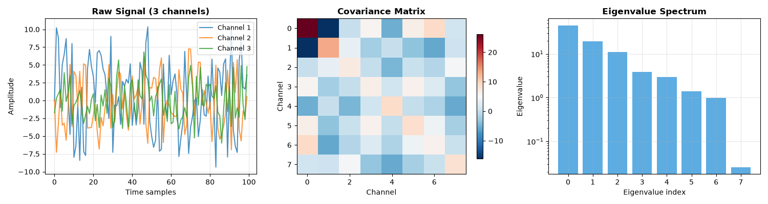
The first step in an SPD network is to compute covariance matrices from raw multivariate signals. Given a signal \(X \in \mathbb{R}^{C \times T}\) with C channels and T time samples, the sample covariance is:

\[\Sigma = \frac{1}{T-1} X X^T\]

This maps the signal from Euclidean space to the SPD manifold.

Input shape: (batch, n_channels, n_times)

Output shape: (batch, n_channels, n_channels)

# Generate synthetic multivariate time series
batch_size = 4
n_channels = 8
n_times = 100

# Create correlated signals
raw_signals = torch.randn(batch_size, n_channels, n_times)

# Add some structure (channel correlations)
mixing_matrix = torch.randn(n_channels, n_channels)
raw_signals = torch.einsum("ij,bjt->bit", mixing_matrix, raw_signals)

print("Input (raw signals):")
print(f"  Shape: {raw_signals.shape}")
print(f"  Min: {raw_signals.min():.3f}, Max: {raw_signals.max():.3f}")

# Apply CovLayer
cov_layer = CovLayer()
covariances = cov_layer(raw_signals)

print("\nOutput (covariance matrices):")
print(f"  Shape: {covariances.shape}")
print(f"  Symmetric: {torch.allclose(covariances, covariances.transpose(-2, -1))}")

# Check positive definiteness
eigvals = torch.linalg.eigvalsh(covariances)
print(f"  Min eigenvalue: {eigvals.min():.6f} (should be > 0 for SPD)")

Input (raw signals):
  Shape: torch.Size([4, 8, 100])
  Min: -13.423, Max: 13.214

Output (covariance matrices):
  Shape: torch.Size([4, 8, 8])
  Symmetric: True
  Min eigenvalue: 0.015668 (should be > 0 for SPD)

Visualizing the Covariance Computation

fig, axes = plt.subplots(1, 3, figsize=(15, 4))

# Plot raw signal (first sample, first 3 channels)
ax1 = axes[0]
time = np.arange(n_times)
for i in range(3):
    ax1.plot(time, raw_signals[0, i, :].numpy(), label=f"Channel {i + 1}", alpha=0.8)
ax1.set_xlabel("Time samples")
ax1.set_ylabel("Amplitude")
ax1.set_title("Raw Signal (3 channels)", fontsize=12, fontweight="bold")
ax1.legend(fontsize=9)
ax1.grid(True, alpha=0.3)

# Plot covariance matrix as heatmap
ax2 = axes[1]
cov_np = covariances[0].numpy()
im = ax2.imshow(cov_np, cmap="RdBu_r", aspect="auto")
ax2.set_title("Covariance Matrix", fontsize=12, fontweight="bold")
ax2.set_xlabel("Channel")
ax2.set_ylabel("Channel")
plt.colorbar(im, ax=ax2, shrink=0.8)

# Plot eigenvalue spectrum
ax3 = axes[2]
eigvals_np = eigvals[0].numpy()
ax3.bar(range(n_channels), sorted(eigvals_np, reverse=True), color="#3498db", alpha=0.8)
ax3.set_xlabel("Eigenvalue index")
ax3.set_ylabel("Eigenvalue")
ax3.set_title("Eigenvalue Spectrum", fontsize=12, fontweight="bold")
ax3.set_yscale("log")
ax3.grid(True, alpha=0.3)

plt.tight_layout()
plt.show()

Block 2: Regularization (Shrinkage & TraceNorm)

Sample covariance matrices can be ill-conditioned, especially when the number of samples is small relative to the number of channels. Regularization improves numerical stability.

Shrinkage (Ledoit-Wolf) [Ledoit and Wolf, 2004]:

\[\Sigma_{reg} = (1 - \alpha) \Sigma + \alpha \cdot \mu \cdot I\]

where \(\alpha\) is the shrinkage coefficient and \(\mu\) is the average eigenvalue (trace / n).

Trace Normalization:

\[\Sigma_{norm} = \frac{\Sigma}{\text{trace}(\Sigma)} + \epsilon I\]

# Apply shrinkage regularization
shrinkage = Shrinkage(n_chans=n_channels, init_shrinkage=0.5, learnable=True)
cov_shrunk = shrinkage(covariances)

# Apply trace normalization
trace_norm = TraceNorm(epsilon=1e-5)
cov_normalized = trace_norm(covariances)

print("Regularization effects:")
print(f"  Original condition number: {torch.linalg.cond(covariances[0]):.1f}")
print(f"  After shrinkage: {torch.linalg.cond(cov_shrunk[0].detach()):.1f}")
print(f"  After trace norm: {torch.linalg.cond(cov_normalized[0]):.1f}")

# Visualize eigenvalue spectra
fig, axes = plt.subplots(1, 3, figsize=(15, 4))

eigvals_orig = torch.linalg.eigvalsh(covariances[0]).numpy()
eigvals_shrunk = torch.linalg.eigvalsh(cov_shrunk[0].detach()).numpy()
eigvals_norm = torch.linalg.eigvalsh(cov_normalized[0]).numpy()

for ax, eigv, title, color in zip(
    axes,
    [eigvals_orig, eigvals_shrunk, eigvals_norm],
    ["Original", "After Shrinkage", "After Trace Norm"],
    ["#3498db", "#e74c3c", "#2ecc71"],
):
    ax.bar(range(n_channels), sorted(eigv, reverse=True), color=color, alpha=0.8)
    ax.set_xlabel("Eigenvalue index")
    ax.set_ylabel("Eigenvalue")
    ax.set_title(title, fontsize=12, fontweight="bold")
    ax.set_yscale("log")
    ax.grid(True, alpha=0.3)
    ax.axhline(y=min(eigv), color="red", linestyle="--", alpha=0.5)
    ax.text(
        n_channels - 1,
        min(eigv) * 1.5,
        f"min={min(eigv):.2e}",
        ha="right",
        fontsize=9,
        color="red",
    )

plt.tight_layout()
plt.show()

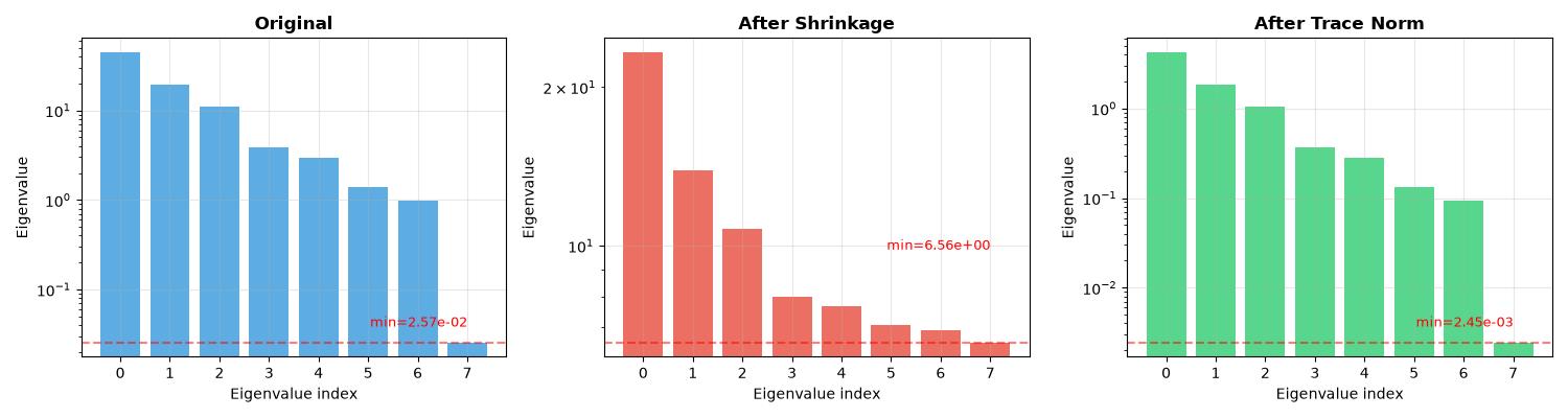
Regularization effects:
  Original condition number: 1724.5
  After shrinkage: 3.6
  After trace norm: 1717.4

Block 3: BiMap Layer

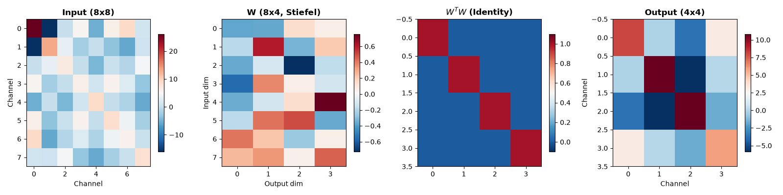
The BiMap (Bilinear Mapping) layer performs dimensionality reduction while preserving the SPD structure. It applies a congruence transformation:

\[Y = W^T X W\]

where \(W \in \mathbb{R}^{n \times m}\) is constrained to lie on the Stiefel manifold (\(W^T W = I\)).

Key properties:

• If X is SPD, then Y is also SPD

• Reduces dimension from n x n to m x m

• W is orthogonal, preventing information collapse

Input shape: (batch, n, n)

Output shape: (batch, m, m)

# Create BiMap layer: reduce from 8x8 to 4x4
bimap = BiMap(in_features=n_channels, out_features=4, parametrized=True)

# Apply BiMap
cov_reduced = bimap(covariances)

print("BiMap transformation:")
print(f"  Input shape: {covariances.shape}")
print(f"  Output shape: {cov_reduced.shape}")
print(f"  Weight matrix W shape: {bimap.weight.shape}")

# Verify orthogonality of W
W = bimap.weight[0]  # Get first (only) weight matrix
WtW = W.T @ W
print("\n  W^T W (should be identity):")
print(f"  {WtW.detach().numpy().round(4)}")

# Verify output is still SPD
eigvals_reduced = torch.linalg.eigvalsh(cov_reduced)
print(
    f"\n  Output eigenvalues (all > 0): {eigvals_reduced[0].detach().numpy().round(4)}"
)

BiMap transformation:
  Input shape: torch.Size([4, 8, 8])
  Output shape: torch.Size([4, 4, 4])
  Weight matrix W shape: torch.Size([1, 8, 4])

  W^T W (should be identity):
  [[ 1. -0.  0.  0.]
 [-0.  1.  0.  0.]
 [ 0.  0.  1. -0.]
 [ 0.  0. -0.  1.]]

  Output eigenvalues (all > 0): [ 2.9852  4.2915 10.4402 17.8522]

Visualizing the BiMap Transformation

fig, axes = plt.subplots(1, 4, figsize=(16, 4))

# Input covariance
ax1 = axes[0]
im1 = ax1.imshow(covariances[0].numpy(), cmap="RdBu_r", aspect="auto")
ax1.set_title("Input (8x8)", fontsize=12, fontweight="bold")
ax1.set_xlabel("Channel")
ax1.set_ylabel("Channel")
plt.colorbar(im1, ax=ax1, shrink=0.8)

# Weight matrix W
ax2 = axes[1]
W_np = bimap.weight[0].detach().numpy()
im2 = ax2.imshow(W_np, cmap="RdBu_r", aspect="auto")
ax2.set_title("W (8x4, Stiefel)", fontsize=12, fontweight="bold")
ax2.set_xlabel("Output dim")
ax2.set_ylabel("Input dim")
plt.colorbar(im2, ax=ax2, shrink=0.8)

# W^T W (should be identity)
ax3 = axes[2]
WtW_np = (W.T @ W).detach().numpy()
im3 = ax3.imshow(WtW_np, cmap="RdBu_r", aspect="auto", vmin=-0.1, vmax=1.1)
ax3.set_title(r"$W^T W$ (Identity)", fontsize=12, fontweight="bold")
plt.colorbar(im3, ax=ax3, shrink=0.8)

# Output covariance
ax4 = axes[3]
im4 = ax4.imshow(cov_reduced[0].detach().numpy(), cmap="RdBu_r", aspect="auto")
ax4.set_title("Output (4x4)", fontsize=12, fontweight="bold")
ax4.set_xlabel("Channel")
ax4.set_ylabel("Channel")
plt.colorbar(im4, ax=ax4, shrink=0.8)

plt.tight_layout()
plt.show()

Block 4: ReEig Layer (Rectified Eigenvalues)

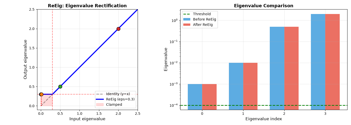
The ReEig layer introduces non-linearity while preserving the SPD property. It applies a ReLU-like function to eigenvalues:

\[\text{ReEig}(X) = U \max(\Lambda, \epsilon) U^T\]

where \(X = U \Lambda U^T\) is the eigendecomposition and \(\epsilon\) is a small threshold.

Geometric interpretation:

• Clamps small eigenvalues to \(\epsilon\)

• Prevents matrices from becoming singular

• Analogous to ReLU in standard neural networks

# Create ReEig layer
reeig = ReEig(threshold=1e-4)

# Create a matrix with some small eigenvalues for demonstration
demo_eigvals = torch.tensor([2.0, 0.5, 0.01, 0.001])
demo_eigvecs = torch.linalg.qr(torch.randn(4, 4))[0]
demo_spd = demo_eigvecs @ torch.diag(demo_eigvals) @ demo_eigvecs.T
demo_spd = demo_spd.unsqueeze(0)  # Add batch dimension

# Apply ReEig
demo_rectified = reeig(demo_spd)

# Compare eigenvalues
eigvals_before = torch.linalg.eigvalsh(demo_spd[0])
eigvals_after = torch.linalg.eigvalsh(demo_rectified[0])

print("ReEig transformation:")
print("  Threshold: 1e-4")
print(f"  Eigenvalues before: {eigvals_before.numpy().round(6)}")
print(f"  Eigenvalues after:  {eigvals_after.numpy().round(6)}")

ReEig transformation:
  Threshold: 1e-4
  Eigenvalues before: [1.e-03 1.e-02 5.e-01 2.e+00]
  Eigenvalues after:  [1.000000e-03 1.000000e-02 5.000000e-01 2.000001e+00]

Visualizing the ReEig Non-linearity

fig, axes = plt.subplots(1, 2, figsize=(14, 5))

# Plot the ReEig function
ax1 = axes[0]
x = np.linspace(0, 2.5, 200)
epsilon = 0.3  # Larger threshold for visualization
y_reeig = np.maximum(x, epsilon)

ax1.plot(x, x, "k--", alpha=0.4, label="Identity (y=x)", linewidth=2)
ax1.plot(x, y_reeig, "b-", linewidth=3, label=f"ReEig (eps={epsilon})")
ax1.fill_between(
    [0, epsilon], [epsilon, epsilon], [0, 0], color="red", alpha=0.15, label="Clamped"
)
ax1.axhline(y=epsilon, color="red", linestyle="--", alpha=0.5)
ax1.axvline(x=epsilon, color="red", linestyle="--", alpha=0.5)

# Mark the demo eigenvalues (scaled for visualization)
scale = 1.0
for i, (ev_before, ev_after) in enumerate(
    zip(eigvals_before.numpy() * scale, eigvals_after.numpy() * scale)
):
    if ev_before < 2.5:
        ax1.scatter(
            [ev_before], [max(ev_before, epsilon)], s=100, zorder=5, edgecolors="black"
        )
        if ev_before < epsilon:
            ax1.plot(
                [ev_before, ev_before],
                [ev_before, epsilon],
                "r:",
                linewidth=2,
                alpha=0.7,
            )

ax1.set_xlim(-0.1, 2.5)
ax1.set_ylim(-0.1, 2.5)
ax1.set_xlabel("Input eigenvalue", fontsize=12)
ax1.set_ylabel("Output eigenvalue", fontsize=12)
ax1.set_title("ReEig: Eigenvalue Rectification", fontsize=13, fontweight="bold")
ax1.legend(loc="lower right", fontsize=10)
ax1.grid(True, alpha=0.3)
ax1.set_aspect("equal")

# Bar plot of eigenvalues
ax2 = axes[1]
x_pos = np.arange(4)
width = 0.35

bars1 = ax2.bar(
    x_pos - width / 2,
    eigvals_before.numpy(),
    width,
    label="Before ReEig",
    color="#3498db",
    alpha=0.8,
)
bars2 = ax2.bar(
    x_pos + width / 2,
    eigvals_after.numpy(),
    width,
    label="After ReEig",
    color="#e74c3c",
    alpha=0.8,
)
ax2.axhline(y=1e-4, color="green", linestyle="--", linewidth=2, label="Threshold")
ax2.set_xlabel("Eigenvalue index", fontsize=12)
ax2.set_ylabel("Eigenvalue", fontsize=12)
ax2.set_title("Eigenvalue Comparison", fontsize=13, fontweight="bold")
ax2.set_yscale("log")
ax2.set_xticks(x_pos)
ax2.legend(fontsize=10)
ax2.grid(True, alpha=0.3)

plt.tight_layout()
plt.show()

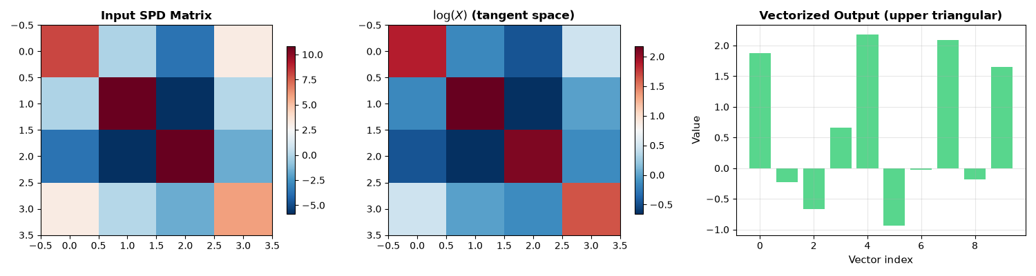
Block 5: LogEig Layer (Logarithmic Map)

The LogEig layer maps SPD matrices to the tangent space at the identity by applying the matrix logarithm:

\[\log(X) = U \log(\Lambda) U^T\]

where \(X = U \Lambda U^T\) is the eigendecomposition.

Geometric interpretation:

• Projects from curved manifold to flat tangent space

• In tangent space, standard Euclidean operations apply

• Output is a symmetric matrix, which can be vectorized

Key insight: The logarithm “flattens” the SPD manifold, allowing us to use standard linear classifiers.

# Create LogEig layer with vectorization
logeig = LogEig(upper=True)

# Use our reduced covariances
log_matrices = logeig(cov_reduced.detach())

print("LogEig transformation:")
print(f"  Input shape: {cov_reduced.shape}")
print(f"  Output shape: {log_matrices.shape}")
print(f"  Output dimension formula: n*(n+1)/2 = 4*5/2 = {4 * 5 // 2}")

LogEig transformation:
  Input shape: torch.Size([4, 4, 4])
  Output shape: torch.Size([4, 10])
  Output dimension formula: n*(n+1)/2 = 4*5/2 = 10

Understanding the Matrix Logarithm

fig, axes = plt.subplots(1, 3, figsize=(15, 4))

# Input SPD matrix
ax1 = axes[0]
spd_input = cov_reduced[0].detach().numpy()
im1 = ax1.imshow(spd_input, cmap="RdBu_r", aspect="auto")
ax1.set_title("Input SPD Matrix", fontsize=12, fontweight="bold")
plt.colorbar(im1, ax=ax1, shrink=0.8)

# Compute full matrix log (without vectorization) for visualization
logeig_full = LogEig(upper=False, flatten=False)
log_full = logeig_full(cov_reduced.detach())

# Matrix logarithm
ax2 = axes[1]
log_matrix = log_full[0].numpy()
im2 = ax2.imshow(log_matrix, cmap="RdBu_r", aspect="auto")
ax2.set_title(r"$\log(X)$ (tangent space)", fontsize=12, fontweight="bold")
plt.colorbar(im2, ax=ax2, shrink=0.8)

# Vectorized output
ax3 = axes[2]
vec_output = log_matrices[0].numpy()
ax3.bar(range(len(vec_output)), vec_output, color="#2ecc71", alpha=0.8)
ax3.set_xlabel("Vector index", fontsize=11)
ax3.set_ylabel("Value", fontsize=11)
ax3.set_title("Vectorized Output (upper triangular)", fontsize=12, fontweight="bold")
ax3.grid(True, alpha=0.3)

plt.tight_layout()
plt.show()

Complete SPDNet Pipeline

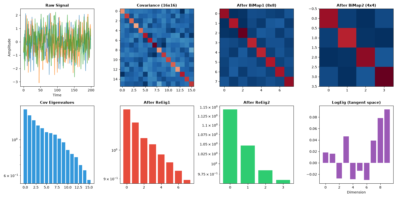
Now let’s put it all together and trace the shape transformations through a complete SPDNet pipeline.

class SimpleSPDNet(nn.Module):
    """A simple SPD network for demonstration."""

    def __init__(self, n_channels, n_classes):
        super().__init__()

        # Layer 1: Covariance computation
        self.cov = CovLayer()

        # Layer 2: Regularization
        self.shrinkage = Shrinkage(n_chans=n_channels, init_shrinkage=0.1)

        # Layer 3: BiMap (reduce dimension)
        self.bimap1 = BiMap(in_features=n_channels, out_features=n_channels // 2)

        # Layer 4: ReEig (non-linearity)
        self.reeig1 = ReEig()

        # Layer 5: Another BiMap
        self.bimap2 = BiMap(in_features=n_channels // 2, out_features=n_channels // 4)

        # Layer 6: Another ReEig
        self.reeig2 = ReEig()

        # Layer 7: LogEig (project to tangent space)
        self.logeig = LogEig(upper=True)

        # Layer 8: Linear classifier
        tangent_dim = (n_channels // 4) * (n_channels // 4 + 1) // 2
        self.classifier = nn.Linear(tangent_dim, n_classes)

    def forward(self, x, return_intermediates=False):
        intermediates = {}

        # Raw signal -> Covariance
        x = self.cov(x)
        intermediates["cov"] = x.clone()

        # Shrinkage regularization
        x = self.shrinkage(x)
        intermediates["shrinkage"] = x.clone()

        # BiMap + ReEig block 1
        x = self.bimap1(x)
        intermediates["bimap1"] = x.clone()
        x = self.reeig1(x)
        intermediates["reeig1"] = x.clone()

        # BiMap + ReEig block 2
        x = self.bimap2(x)
        intermediates["bimap2"] = x.clone()
        x = self.reeig2(x)
        intermediates["reeig2"] = x.clone()

        # LogEig (to tangent space)
        x = self.logeig(x)
        intermediates["logeig"] = x.clone()

        # Linear classifier
        x = self.classifier(x)
        intermediates["output"] = x.clone()

        if return_intermediates:
            return x, intermediates
        return x


# Create and use the network
n_channels = 16
n_classes = 4
model = SimpleSPDNet(n_channels=n_channels, n_classes=n_classes)

# Generate input
batch_size = 8
n_times = 200
raw_input = torch.randn(batch_size, n_channels, n_times)

# Forward pass with intermediates
output, intermediates = model(raw_input, return_intermediates=True)

# Print shape transformations
print("Shape Transformations Through SPDNet")
print("=" * 50)
print(f"Input (raw signal):     {raw_input.shape}")
print(f"After CovLayer:         {intermediates['cov'].shape}")
print(f"After Shrinkage:        {intermediates['shrinkage'].shape}")
print(f"After BiMap1 (16->8):   {intermediates['bimap1'].shape}")
print(f"After ReEig1:           {intermediates['reeig1'].shape}")
print(f"After BiMap2 (8->4):    {intermediates['bimap2'].shape}")
print(f"After ReEig2:           {intermediates['reeig2'].shape}")
print(f"After LogEig:           {intermediates['logeig'].shape}")
print(f"Output (logits):        {output.shape}")

Shape Transformations Through SPDNet
==================================================
Input (raw signal):     torch.Size([8, 16, 200])
After CovLayer:         torch.Size([8, 16, 16])
After Shrinkage:        torch.Size([8, 16, 16])
After BiMap1 (16->8):   torch.Size([8, 8, 8])
After ReEig1:           torch.Size([8, 8, 8])
After BiMap2 (8->4):    torch.Size([8, 4, 4])
After ReEig2:           torch.Size([8, 4, 4])
After LogEig:           torch.Size([8, 10])
Output (logits):        torch.Size([8, 4])

Visualizing the Full Pipeline

fig, axes = plt.subplots(2, 4, figsize=(16, 8))

# Row 1: Matrix representations
ax1 = axes[0, 0]
ax1.plot(raw_input[0, :3, :].T.numpy(), alpha=0.7)
ax1.set_title("Raw Signal", fontsize=11, fontweight="bold")
ax1.set_xlabel("Time")
ax1.set_ylabel("Amplitude")

ax2 = axes[0, 1]
im2 = ax2.imshow(intermediates["cov"][0].detach().numpy(), cmap="RdBu_r", aspect="auto")
ax2.set_title("Covariance (16x16)", fontsize=11, fontweight="bold")

ax3 = axes[0, 2]
im3 = ax3.imshow(
    intermediates["bimap1"][0].detach().numpy(), cmap="RdBu_r", aspect="auto"
)
ax3.set_title("After BiMap1 (8x8)", fontsize=11, fontweight="bold")

ax4 = axes[0, 3]
im4 = ax4.imshow(
    intermediates["bimap2"][0].detach().numpy(), cmap="RdBu_r", aspect="auto"
)
ax4.set_title("After BiMap2 (4x4)", fontsize=11, fontweight="bold")

# Row 2: Eigenvalue spectra and output
ax5 = axes[1, 0]
eigvals_cov = torch.linalg.eigvalsh(intermediates["cov"][0]).numpy()
ax5.bar(range(len(eigvals_cov)), sorted(eigvals_cov, reverse=True), color="#3498db")
ax5.set_title("Cov Eigenvalues", fontsize=11, fontweight="bold")
ax5.set_yscale("log")

ax6 = axes[1, 1]
eigvals_bimap1 = torch.linalg.eigvalsh(intermediates["reeig1"][0]).detach().numpy()
ax6.bar(
    range(len(eigvals_bimap1)), sorted(eigvals_bimap1, reverse=True), color="#e74c3c"
)
ax6.set_title("After ReEig1", fontsize=11, fontweight="bold")
ax6.set_yscale("log")

ax7 = axes[1, 2]
eigvals_bimap2 = torch.linalg.eigvalsh(intermediates["reeig2"][0]).detach().numpy()
ax7.bar(
    range(len(eigvals_bimap2)), sorted(eigvals_bimap2, reverse=True), color="#2ecc71"
)
ax7.set_title("After ReEig2", fontsize=11, fontweight="bold")
ax7.set_yscale("log")

ax8 = axes[1, 3]
logeig_vec = intermediates["logeig"][0].detach().numpy()
ax8.bar(range(len(logeig_vec)), logeig_vec, color="#9b59b6")
ax8.set_title("LogEig (tangent space)", fontsize=11, fontweight="bold")
ax8.set_xlabel("Dimension")

plt.tight_layout()
plt.show()

Composing Custom Architectures

The modular design of SPD Learn allows flexible architecture composition. Here are some common patterns:

class DeepSPDNet(nn.Module):
    """Deeper SPD network with multiple BiMap+ReEig blocks."""

    def __init__(self, n_channels, hidden_dims, n_classes):
        super().__init__()

        self.cov = CovLayer()
        self.shrinkage = Shrinkage(n_chans=n_channels)

        # Build BiMap+ReEig blocks
        self.blocks = nn.ModuleList()
        dims = [n_channels] + list(hidden_dims)
        for i in range(len(hidden_dims)):
            self.blocks.append(
                nn.Sequential(
                    BiMap(in_features=dims[i], out_features=dims[i + 1]),
                    ReEig(),
                )
            )

        self.logeig = LogEig(upper=True)
        final_dim = hidden_dims[-1] * (hidden_dims[-1] + 1) // 2
        self.classifier = nn.Linear(final_dim, n_classes)

    def forward(self, x):
        x = self.cov(x)
        x = self.shrinkage(x)

        for block in self.blocks:
            x = block(x)

        x = self.logeig(x)
        return self.classifier(x)


# Create a deeper network
deep_model = DeepSPDNet(
    n_channels=22,  # EEG with 22 channels
    hidden_dims=[16, 8, 4],  # Progressive reduction
    n_classes=4,  # 4-class motor imagery
)

# Count parameters
n_params = sum(p.numel() for p in deep_model.parameters())
print("\nDeepSPDNet Architecture:")
print("  Input channels: 22")
print("  Hidden dimensions: 22 -> 16 -> 8 -> 4")
print(f"  Output features: {4 * 5 // 2} (vectorized)")
print(f"  Total parameters: {n_params:,}")

DeepSPDNet Architecture:
  Input channels: 22
  Hidden dimensions: 22 -> 16 -> 8 -> 4
  Output features: 10 (vectorized)
  Total parameters: 557

Summary: The SPD Learning Pipeline

This tutorial covered the fundamental building blocks of SPD neural networks:

1. CovLayer: Transforms raw signals to SPD covariance matrices

2. Shrinkage/TraceNorm: Regularizes covariance matrices for stability

3. BiMap: Performs geometry-preserving dimensionality reduction using orthogonal projections

4. ReEig: Introduces non-linearity by rectifying eigenvalues, analogous to ReLU in standard networks

5. LogEig: Maps SPD matrices to tangent space where Euclidean operations apply, enabling standard linear classification

Key insights:

• All operations preserve SPD structure until LogEig

• BiMap uses Stiefel manifold constraints for stable training [Brooks et al., 2019]

• The pipeline gradually reduces dimensionality while preserving information

• LogEig “flattens” the manifold for classification

For more advanced architectures, see the EEGSPDNet and TSMNet tutorials.