
Note
Go to the end to download the full example code.
Manifold Attention with MAtt#
This tutorial demonstrates how to use MAtt (Manifold Attention Network) for EEG classification. MAtt applies attention mechanisms on the SPD manifold to weight temporal segments by their discriminative importance.
Introduction#
MAtt [Pan et al., 2022] introduces attention mechanisms on the SPD manifold:
Patch-based Processing: Segments the signal into temporal patches
Covariance per Patch: Computes SPD matrices for each segment
Manifold Attention: Weights patches using Log-Euclidean distances
Aggregation: Combines weighted SPD matrices for classification
This allows the model to focus on the most discriminative time periods within each trial, improving classification and interpretability.
Setup and Imports#
import warnings

import matplotlib.pyplot as plt
import torch

from braindecode import EEGClassifier
from moabb.datasets import BNCI2014_001
from moabb.paradigms import MotorImagery
from sklearn.metrics import accuracy_score
from sklearn.preprocessing import LabelEncoder
from skorch.callbacks import EpochScoring, GradientNormClipping
from skorch.dataset import ValidSplit

from spd_learn.models import MAtt


warnings.filterwarnings("ignore")
/opt/hostedtoolcache/Python/3.11.16/x64/lib/python3.11/site-packages/braindecode/models/eegpt.py:497: FutureWarning: Montage name 'standard_1020' is deprecated and will be removed in MNE 1.14. Use 'colin27_1020' instead.
  montage = mne.channels.make_standard_montage("standard_1020")
/opt/hostedtoolcache/Python/3.11.16/x64/lib/python3.11/site-packages/braindecode/models/eegpt.py:1452: FutureWarning: Montage name 'standard_1020' is deprecated and will be removed in MNE 1.14. Use 'colin27_1020' instead.
  montage = make_standard_montage("standard_1020")
Loading the Dataset#
dataset = BNCI2014_001()
paradigm = MotorImagery(n_classes=4)

print(f"Dataset: {dataset.code}")
print("Paradigm: 4-class motor imagery")
Choosing from all possible events
Dataset: BNCI2014-001
Paradigm: 4-class motor imagery
Creating the MAtt Model#
MAtt architecture:
Spatial Conv: Learns spatial filters
Temporal Conv: Extracts temporal features
Patch Embedding: Segments into n_patches temporal windows
Covariance + TraceNorm: SPD matrix per patch
AttentionManifold: Queries, keys, values on SPD manifold
ReEig + LogEig: Project to tangent space
Linear: Classification
The attention mechanism computes:
where \(d_{LE}\) is the Log-Euclidean distance.
n_chans = 22
n_outputs = 4

model = MAtt(
    n_chans=n_chans,
    n_outputs=n_outputs,
    n_patches=6,  # Number of temporal segments
    temporal_out_channels=32,  # Temporal feature dimension
    temporal_kernel_size=25,  # ~100ms at 250Hz
    temporal_padding=12,  # Keep time dimension
    attention_in_features=32,  # Input to attention (must match temporal_out_channels)
    attention_out_features=24,  # Output from attention
)

print("MAtt Architecture:")
print(model)
MAtt Architecture:
MAtt(
  (add_extra_dim): Rearrange('batch chan time -> batch 1 chan time')
  (spatial_filter): Conv2d(1, 22, kernel_size=(22, 1), stride=(1, 1))
  (spatial_batch_norm): BatchNorm2d(22, eps=1e-05, momentum=0.1, affine=True, bias=True, track_running_stats=True)
  (temporal_feature_extractor): Conv2d(22, 32, kernel_size=(1, 25), stride=(1, 1), padding=(0, 12))
  (temporal_batch_norm): BatchNorm2d(32, eps=1e-05, momentum=0.1, affine=True, bias=True, track_running_stats=True)
  (squeeze_channel): Rearrange('batch kernel 1 time -> batch kernel time')
  (patch_cov_layer): Sequential(
    (0): PatchEmbeddingLayer()
    (1): CovLayer()
    (2): TraceNorm()
  )
  (manifold_attention): AttentionManifold(
    (q_trans): ParametrizedBiMap(
      (parametrizations): ModuleDict(
        (weight): ParametrizationList(
          (0): _Orthogonal()
        )
      )
    )
    (k_trans): ParametrizedBiMap(
      (parametrizations): ModuleDict(
        (weight): ParametrizationList(
          (0): _Orthogonal()
        )
      )
    )
    (v_trans): ParametrizedBiMap(
      (parametrizations): ModuleDict(
        (weight): ParametrizationList(
          (0): _Orthogonal()
        )
      )
    )
  )
  (re_eig): ReEig()
  (tangent): LogEig()
  (flatten): Flatten(start_dim=1, end_dim=-1)
  (linear): Linear(in_features=1800, out_features=4, bias=True)
)
Training the Model#
subject_id = 1
batch_size = 32
max_epochs = 100
learning_rate = 1e-4  # Low learning rate for stable SPD learning

device = "cuda" if torch.cuda.is_available() else "cpu"
print(f"\nUsing device: {device}")

# Cache configuration
cache_config = dict(
    save_raw=True,
    save_epochs=True,
    save_array=True,
    use=True,
    overwrite_raw=False,
    overwrite_epochs=False,
    overwrite_array=False,
)

# Load data
X, labels, meta = paradigm.get_data(
    dataset=dataset, subjects=[subject_id], cache_config=cache_config
)

# Encode labels
le = LabelEncoder()
y = le.fit_transform(labels)

# Split by session
train_idx = meta.query("session == '0train'").index.to_numpy()
test_idx = meta.query("session == '1test'").index.to_numpy()

print(f"\nData shape: {X.shape}")
print(f"Training samples: {len(train_idx)}")
print(f"Test samples: {len(test_idx)}")

# Create classifier
# Note: SPD networks benefit from gradient clipping to prevent
# divergence during training on the Riemannian manifold.
clf = EEGClassifier(
    model,
    criterion=torch.nn.CrossEntropyLoss,
    optimizer=torch.optim.Adam,
    optimizer__lr=learning_rate,
    train_split=ValidSplit(0.1, stratified=True, random_state=42),
    batch_size=batch_size,
    max_epochs=max_epochs,
    callbacks=[
        (
            "train_acc",
            EpochScoring(
                "accuracy", lower_is_better=False, on_train=True, name="train_acc"
            ),
        ),
        ("gradient_clip", GradientNormClipping(gradient_clip_value=1.0)),
    ],
    device=device,
    verbose=1,
)

# Train
clf.fit(X[train_idx], y[train_idx])

# Evaluate
y_pred_train = clf.predict(X[train_idx])
y_pred_test = clf.predict(X[test_idx])

train_acc = accuracy_score(y[train_idx], y_pred_train)
test_acc = accuracy_score(y[test_idx], y_pred_test)

print(f"\n{'=' * 50}")
print(f"Results for Subject {subject_id}")
print(f"{'=' * 50}")
print(f"Train Accuracy: {train_acc * 100:.2f}%")
print(f"Test Accuracy:  {test_acc * 100:.2f}%")
Using device: cpu

Data shape: (576, 22, 1001)
Training samples: 288
Test samples: 288
  epoch    train_acc    train_loss    valid_acc    valid_loss     dur
-------  -----------  ------------  -----------  ------------  ------
      1       0.2461        1.3908       0.2759        1.3606  1.7426
      2       0.3945        1.3495       0.5517        1.3219  1.6389
      3       0.4648        1.3113       0.4138        1.2982  1.6662
      4       0.4062        1.2886       0.2414        1.2887  2.1601
      5       0.5156        1.2544       0.4483        1.2515  1.7126
      6       0.6016        1.2276       0.5517        1.2235  1.6299
      7       0.5781        1.2027       0.4828        1.2100  1.6211
      8       0.6250        1.1694       0.5517        1.1703  1.6345
      9       0.6602        1.1467       0.6207        1.1627  1.6325
     10       0.6602        1.1217       0.5517        1.1392  1.6524
     11       0.7031        1.0933       0.5862        1.1016  1.6330
     12       0.7109        1.0606       0.7241        1.0879  1.6331
     13       0.7500        1.0349       0.6552        1.0681  1.6705
     14       0.7617        1.0160       0.7241        1.0392  1.6376
     15       0.7227        0.9906       0.6207        1.0224  1.6497
     16       0.7812        0.9618       0.6552        1.0031  1.6358
     17       0.7539        0.9419       0.7241        0.9797  1.6381
     18       0.7852        0.9120       0.6552        0.9591  1.6309
     19       0.8203        0.8814       0.7931        0.9389  1.6607
     20       0.7656        0.8752       0.7241        0.9340  1.6420
     21       0.7773        0.8537       0.6207        0.9085  1.6379
     22       0.7812        0.8287       0.7241        0.8961  1.6586
     23       0.7734        0.8143       0.6897        0.8852  1.6457
     24       0.8320        0.7869       0.6552        0.8728  1.6359
     25       0.8281        0.7810       0.7931        0.8583  1.6238
     26       0.8242        0.7705       0.7931        0.8581  1.6366
     27       0.8516        0.7459       0.7931        0.8280  1.6341
     28       0.8359        0.7386       0.8276        0.8395  1.6288
     29       0.8359        0.7254       0.8966        0.8095  1.6307
     30       0.8359        0.7227       0.6552        0.8541  1.6504
     31       0.8516        0.7072       0.7586        0.7926  1.6611
     32       0.8281        0.6863       0.7931        0.8066  1.6448
     33       0.8359        0.6887       0.6552        0.8013  1.6413
     34       0.8555        0.6717       0.8621        0.7707  1.6539
     35       0.8320        0.6577       0.7931        0.7988  1.6493
     36       0.8359        0.6457       0.7931        0.7603  1.6516
     37       0.8711        0.6312       0.8621        0.7607  1.6679
     38       0.8672        0.6256       0.7931        0.7580  1.6605
     39       0.8438        0.6211       0.7586        0.7511  1.6564
     40       0.8516        0.6058       0.8966        0.7455  1.6624
     41       0.8555        0.6041       0.7586        0.7433  1.6352
     42       0.8750        0.5953       0.7931        0.7342  1.6656
     43       0.8906        0.5758       0.7586        0.7277  1.6841
     44       0.8828        0.5690       0.8276        0.7336  1.6813
     45       0.8750        0.5612       0.7931        0.7009  1.6521
     46       0.8828        0.5493       0.8621        0.7178  1.6788
     47       0.8750        0.5463       0.8966        0.6946  1.6287
     48       0.8945        0.5351       0.7586        0.7092  1.6687
     49       0.8516        0.5423       0.8621        0.6876  1.6905
     50       0.9023        0.5094       0.7586        0.7083  1.6453
     51       0.9102        0.5078       0.8621        0.6716  1.6767
     52       0.8828        0.5043       0.8966        0.6733  1.6555
     53       0.9102        0.4897       0.8276        0.6781  1.6502
     54       0.8906        0.5020       0.8276        0.6604  1.6789
     55       0.9102        0.4948       0.7586        0.6932  1.6623
     56       0.8906        0.4893       0.6207        0.6755  1.6531
     57       0.8945        0.4805       0.7586        0.6830  1.6496
     58       0.8867        0.4780       0.8621        0.6571  1.6788
     59       0.9141        0.4763       0.7931        0.6554  1.6766
     60       0.8984        0.4576       0.7931        0.6795  1.6789
     61       0.9180        0.4471       0.8276        0.6424  1.6505
     62       0.9414        0.4399       0.8966        0.6446  1.6774
     63       0.9062        0.4424       0.8966        0.6284  1.6470
     64       0.9375        0.4239       0.8621        0.6375  1.6941
     65       0.8984        0.4321       0.7931        0.6497  1.6594
     66       0.9297        0.4216       0.8966        0.6145  1.6729
     67       0.9297        0.4159       0.8276        0.6443  1.6555
     68       0.9375        0.4029       0.8276        0.6233  2.2558
     69       0.9414        0.4079       0.8621        0.6276  2.3638
     70       0.9414        0.4028       0.8621        0.6098  2.3725
     71       0.9336        0.3892       0.8276        0.6299  2.3674
     72       0.9336        0.3897       0.8621        0.5963  2.3711
     73       0.9336        0.3863       0.8621        0.6087  2.3558
     74       0.9609        0.3736       0.8966        0.5968  2.3698
     75       0.9492        0.3715       0.7931        0.6019  2.3711
     76       0.9492        0.3650       0.7586        0.6299  2.3719
     77       0.9375        0.3611       0.8966        0.5870  2.3150
     78       0.9414        0.3548       0.8276        0.6108  1.9148
     79       0.9570        0.3533       0.8276        0.6006  1.6505
     80       0.9570        0.3449       0.8621        0.5979  1.6482
     81       0.9727        0.3411       0.8276        0.5920  1.7066
     82       0.9648        0.3339       0.9310        0.5847  1.6578
     83       0.9766        0.3333       0.8276        0.6050  1.6739
     84       0.9570        0.3316       0.9310        0.5625  1.6658
     85       0.9492        0.3336       0.8276        0.5848  1.6561
     86       0.9648        0.3156       0.8621        0.5773  1.6634
     87       0.9727        0.3100       0.8621        0.5654  1.6623
     88       0.9805        0.3115       0.7586        0.6136  1.6736
     89       0.9727        0.3152       0.8621        0.5562  1.6560
     90       0.9648        0.3038       0.8276        0.6002  1.6744
     91       0.9766        0.3060       0.8621        0.5691  1.6672
     92       0.9531        0.3080       0.8276        0.5625  1.6633
     93       0.9805        0.2949       0.8966        0.5702  1.6363
     94       0.9844        0.2913       0.7931        0.5886  1.6518
     95       0.9727        0.2844       0.7241        0.6108  1.6990
     96       0.9766        0.2835       0.7931        0.5682  1.6571
     97       0.9727        0.2749       0.7241        0.5966  1.7396
     98       0.9766        0.2821       0.8276        0.5495  1.6674
     99       0.9766        0.2761       0.8276        0.5578  1.8198
    100       0.9844        0.2668       0.8276        0.5599  1.6783

==================================================
Results for Subject 1
==================================================
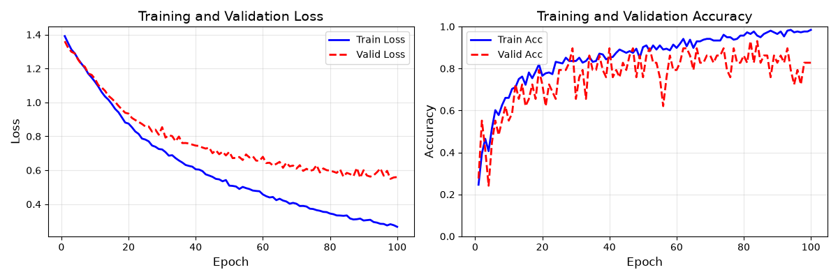
Train Accuracy: 97.57%
Test Accuracy:  79.51%
Visualizing Results#
fig, axes = plt.subplots(1, 2, figsize=(12, 4))

# Training history
history = clf.history
epochs = range(1, len(history) + 1)

ax1 = axes[0]
ax1.plot(epochs, history[:, "train_loss"], "b-", label="Train Loss", linewidth=2)
ax1.plot(epochs, history[:, "valid_loss"], "r--", label="Valid Loss", linewidth=2)
ax1.set_xlabel("Epoch", fontsize=12)
ax1.set_ylabel("Loss", fontsize=12)
ax1.set_title("Training and Validation Loss", fontsize=14)
ax1.legend(fontsize=10)
ax1.grid(True, alpha=0.3)

ax2 = axes[1]
ax2.plot(epochs, history[:, "train_acc"], "b-", label="Train Acc", linewidth=2)
ax2.plot(epochs, history[:, "valid_acc"], "r--", label="Valid Acc", linewidth=2)
ax2.set_xlabel("Epoch", fontsize=12)
ax2.set_ylabel("Accuracy", fontsize=12)
ax2.set_title("Training and Validation Accuracy", fontsize=14)
ax2.legend(fontsize=10)
ax2.grid(True, alpha=0.3)
ax2.set_ylim([0, 1])

plt.tight_layout()
plt.show()
Understanding Manifold Attention#
The attention mechanism in MAtt operates differently from standard attention:
Standard Attention (Euclidean):
Manifold Attention (Log-Euclidean):
This respects the Riemannian geometry of SPD matrices, computing meaningful distances on the manifold rather than in Euclidean space.
Summary#
In this tutorial, we demonstrated:
Creating a MAtt model with patch-based temporal segmentation
Training for motor imagery classification
Understanding the manifold attention mechanism
MAtt is particularly useful when:
Different time segments have varying discriminative power
You want interpretable attention weights
The data has complex temporal dynamics
Total running time of the script: (2 minutes 59.501 seconds)
