How to Choose a Metric for Batch Normalization

Select the right Riemannian metric for SPDBatchNormLie. Each metric trades off speed, invariance, and numerical stability.

Prerequisites: Familiarity with SPD batch normalization (see Batch Normalization on SPD Manifolds).

Quick Decision Guide

Metric	Speed	Invariance	Use When
LEM	Fastest	Orthogonal	Default choice. Closed-form mean, good general performance.
AIM	Slowest	Full affine	Data has varying scale (e.g., cross-subject EEG).
LCM	Fast	Lower-triangular	Speed matters and you want Cholesky stability.

import time

import matplotlib.pyplot as plt
import numpy as np
import torch

from pyriemann.datasets import make_gaussian_blobs

from spd_learn.modules import SPDBatchNormLie


torch.manual_seed(42)

# Generate SPD data using pyriemann (2-class, 2*n_matrices total samples)
n_matrices = 32
n_dim = 8
X_np, y = make_gaussian_blobs(
    n_matrices=n_matrices,
    n_dim=n_dim,
    class_sep=1.5,
    class_disp=0.5,
    random_state=42,
)
X = torch.from_numpy(X_np).float()  # shape: (64, 8, 8)

metric_colors = {"LEM": "#2ecc71", "LCM": "#3498db", "AIM": "#e74c3c"}

Comparing Forward Pass Speed

The cost depends on the metric’s mean computation. AIM requires an iterative Karcher mean, while LEM and LCM use closed-form means. We use larger 32x32 matrices here so timing differences are visible.

n_bench = 32
batch_size = 64
A = torch.randn(batch_size, n_bench, n_bench)
X_bench = A @ A.mT + 0.01 * torch.eye(n_bench)

timings = {}
for metric in ["LEM", "LCM", "AIM"]:
    bn = SPDBatchNormLie(n_bench, metric=metric)
    bn.train()
    _ = bn(X_bench)  # warmup
    t0 = time.time()
    for _ in range(20):
        _ = bn(X_bench)
    elapsed = (time.time() - t0) / 20
    timings[metric] = elapsed * 1000
    print(
        f"{metric}: {elapsed * 1000:.1f} ms/batch ({n_bench}x{n_bench}, batch={batch_size})"
    )

fig, ax = plt.subplots(figsize=(6, 4))
ax.bar(
    timings.keys(),
    timings.values(),
    color=[metric_colors[m] for m in timings],
)
ax.set_ylabel("Time (ms)")
ax.set_title("Forward Pass Speed by Metric")
ax.grid(axis="y", alpha=0.3)
plt.tight_layout()
plt.show()

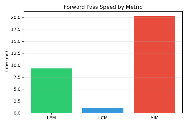
LEM: 9.3 ms/batch (32x32, batch=64)
LCM: 1.1 ms/batch (32x32, batch=64)
AIM: 20.2 ms/batch (32x32, batch=64)

Comparing Output Properties

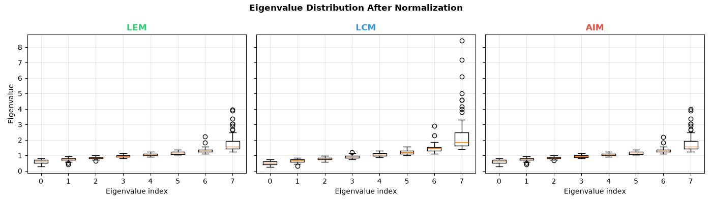
Each metric normalizes eigenvalues differently. Inspect the eigenvalue distribution after normalization:

fig, axes = plt.subplots(1, 3, figsize=(14, 4), sharey=True)
for ax, metric in zip(axes, ["LEM", "LCM", "AIM"]):
    bn = SPDBatchNormLie(n_dim, metric=metric)
    bn.train()
    Y = bn(X)
    eigvals = torch.linalg.eigvalsh(Y.detach())
    ax.boxplot(
        [eigvals[:, i].numpy() for i in range(n_dim)],
        positions=range(n_dim),
    )
    ax.set_title(f"{metric}", color=metric_colors[metric], fontweight="bold")
    ax.set_xlabel("Eigenvalue index")
    ax.grid(True, alpha=0.3)

axes[0].set_ylabel("Eigenvalue")
plt.suptitle("Eigenvalue Distribution After Normalization", fontweight="bold")
plt.tight_layout()
plt.show()

Effect of Each Metric on an SPD Matrix

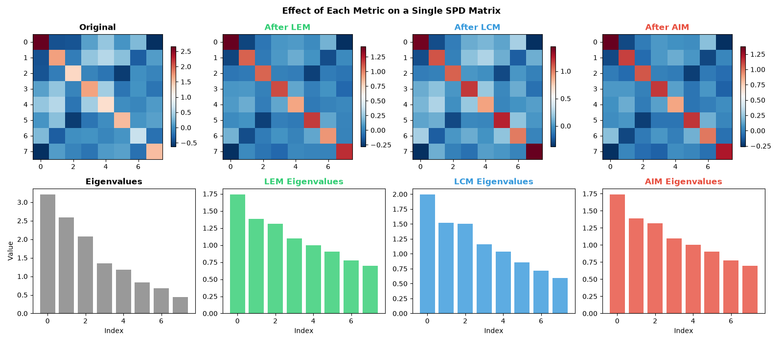
To build visual intuition, let’s examine how each metric transforms a single SPD matrix. The top row shows the matrix entries as a heatmap (before and after normalization), while the bottom row compares the eigenvalue spectrum.

sample_idx = 0
X_sample = X[sample_idx]  # shape (8, 8)

fig, axes = plt.subplots(2, 4, figsize=(16, 7))

# Top row: matrix heatmaps
im = axes[0, 0].imshow(X_sample.numpy(), cmap="RdBu_r", aspect="auto")
axes[0, 0].set_title("Original", fontweight="bold")
plt.colorbar(im, ax=axes[0, 0], shrink=0.8)

normalized = {}
for col, metric in enumerate(["LEM", "LCM", "AIM"], start=1):
    bn = SPDBatchNormLie(n_dim, metric=metric)
    bn.train()
    Y = bn(X)
    Y_sample = Y[sample_idx].detach().numpy()
    normalized[metric] = Y_sample

    ax = axes[0, col]
    im = ax.imshow(Y_sample, cmap="RdBu_r", aspect="auto")
    ax.set_title(f"After {metric}", fontweight="bold", color=metric_colors[metric])
    plt.colorbar(im, ax=ax, shrink=0.8)

# Bottom row: eigenvalue bar charts
eigvals_orig = np.sort(np.linalg.eigvalsh(X_sample.numpy()))[::-1]
axes[1, 0].bar(range(n_dim), eigvals_orig, color="gray", alpha=0.8)
axes[1, 0].set_title("Eigenvalues", fontweight="bold")
axes[1, 0].set_xlabel("Index")
axes[1, 0].set_ylabel("Value")

for col, metric in enumerate(["LEM", "LCM", "AIM"], start=1):
    eigvals_after = np.sort(np.linalg.eigvalsh(normalized[metric]))[::-1]
    ax = axes[1, col]
    ax.bar(
        range(n_dim),
        eigvals_after,
        color=metric_colors[metric],
        alpha=0.8,
    )
    ax.set_title(
        f"{metric} Eigenvalues", fontweight="bold", color=metric_colors[metric]
    )
    ax.set_xlabel("Index")

plt.suptitle(
    "Effect of Each Metric on a Single SPD Matrix",
    fontweight="bold",
    fontsize=13,
)
plt.tight_layout()
plt.show()

Tuning the Theta Parameter

The theta parameter controls the power deformation \(P^\theta\). It adjusts how strongly scale differences are compressed or amplified:

• theta=0.5: Square root – compresses large scale differences

• theta=1.0: No deformation (default)

• theta=1.5: Amplifies scale differences

The violin plots below show how the eigenvalue distribution changes with each theta value under the AIM metric:

thetas = [0.5, 1.0, 1.5]
theta_colors = ["#3498db", "#9b59b6", "#f39c12"]

fig, axes = plt.subplots(1, 3, figsize=(14, 4), sharey=True)

for ax, theta, color in zip(axes, thetas, theta_colors):
    bn = SPDBatchNormLie(n_dim, metric="AIM", theta=theta)
    bn.train()
    Y = bn(X)
    eigvals = torch.linalg.eigvalsh(Y.detach()).numpy()

    parts = ax.violinplot(
        [eigvals[:, i] for i in range(n_dim)],
        positions=range(n_dim),
        showmedians=True,
        showextrema=True,
    )
    for pc in parts["bodies"]:
        pc.set_facecolor(color)
        pc.set_alpha(0.6)
    for key in ("cbars", "cmins", "cmaxes", "cmedians"):
        parts[key].set_color(color)

    ax.set_title(f"θ = {theta}", fontweight="bold", fontsize=12)
    ax.set_xlabel("Eigenvalue index")
    ax.grid(True, alpha=0.3)

    print(
        f"AIM (theta={theta}): eigval range [{eigvals.min():.3f}, {eigvals.max():.3f}]"
    )

axes[0].set_ylabel("Eigenvalue")
plt.suptitle(
    "Theta Parameter Effect on Eigenvalue Distribution (AIM Metric)",
    fontweight="bold",
)
plt.tight_layout()
plt.show()

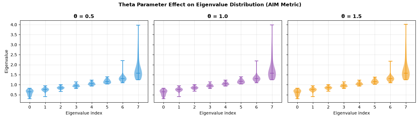
AIM (theta=0.5): eigval range [0.300, 3.975]
AIM (theta=1.0): eigval range [0.299, 3.987]
AIM (theta=1.5): eigval range [0.298, 4.019]

Recommendations

1. Start with LEM – fastest, closed-form mean, works well in most cases

2. Try AIM if your data has varying scale across subjects or sessions

3. Use LCM when you need speed similar to LEM with Cholesky stability

4. Tune theta on a validation set when using AIM or LCM (see Reproducing LieBN Paper Results (Table 4) for a multi-dataset benchmark)

See also

• Batch Normalization on SPD Manifolds – Detailed tutorial on SPD BN

• How to Add Batch Normalization to an SPDNet – How to add BN to your pipeline

• Reproducing LieBN Paper Results (Table 4) – Full benchmark reproduction

• SPDBatchNormLie – API reference