
Note
Go to the end to download the full example code.
Batch Normalization on SPD Manifolds#
This tutorial teaches how batch normalization works on SPD matrices and why it matters for training SPD neural networks. You will train a simple SPDNet with and without normalization, observe the impact, and compare different Riemannian metrics.
By the end, you will understand:
Why standard Euclidean batch normalization doesn’t apply to SPD matrices
How Riemannian and Lie group batch normalization work
When to use each metric (AIM, LEM, LCM)
Setup and Imports#
import matplotlib.pyplot as plt
import numpy as np
import torch
import torch.nn as nn

from spd_learn.modules import (
    BiMap,
    LogEig,
    ReEig,
    SPDBatchNormLie,
    SPDBatchNormMeanVar,
)


torch.manual_seed(42)
np.random.seed(42)
Creating Synthetic SPD Data#
We generate a 3-class classification problem with 8x8 SPD matrices. Each class has a distinct eigenvalue profile, simulating how real-world signals (EEG, radar) produce covariance matrices with different spectral characteristics.
def make_spd_dataset(n_samples_per_class=100, n=8, n_classes=3, seed=42):
    """Generate synthetic SPD classification data."""
    rng = np.random.RandomState(seed)
    X_list, y_list = [], []
    for c in range(n_classes):
        eigvals = np.exp(rng.randn(n) * 0.5 + c * 0.3)
        for _ in range(n_samples_per_class):
            Q, _ = np.linalg.qr(rng.randn(n, n))
            S = Q @ np.diag(eigvals + rng.rand(n) * 0.1) @ Q.T
            S = (S + S.T) / 2
            X_list.append(S)
            y_list.append(c)
    X = torch.from_numpy(np.stack(X_list)).float()
    y = torch.from_numpy(np.array(y_list))
    perm = torch.randperm(len(X), generator=torch.Generator().manual_seed(seed))
    return X[perm], y[perm]


X, y = make_spd_dataset()
n_train = int(0.7 * len(X))
X_train, y_train = X[:n_train], y[:n_train]
X_test, y_test = X[n_train:], y[n_train:]
print(
    f"Dataset: {len(X)} samples ({n_train} train, {len(X) - n_train} test), "
    f"{len(torch.unique(y))} classes, {X.shape[1]}x{X.shape[2]} SPD matrices"
)
Dataset: 300 samples (210 train, 90 test), 3 classes, 8x8 SPD matrices
A Simple SPDNet#
We define a minimal SPDNet with one BiMap layer, optional batch normalization, ReEig activation, and a LogEig + linear classifier.
class SimpleSPDNet(nn.Module):
    """Minimal SPDNet with optional batch normalization."""

    def __init__(self, n_in, n_out, n_classes, bn=None):
        super().__init__()
        self.bimap = BiMap(n_in, n_out)
        self.bn = bn
        self.reeig = ReEig()
        self.logeig = LogEig(upper=False, flatten=True)
        self.classifier = nn.Linear(n_out**2, n_classes)

    def forward(self, x):
        x = self.bimap(x)
        if self.bn is not None:
            x = self.bn(x)
        x = self.reeig(x)
        x = self.logeig(x)
        return self.classifier(x)


def train_model(model, X_train, y_train, X_test, y_test, epochs=150, lr=5e-3):
    """Train a model and record loss and accuracy curves."""
    optimizer = torch.optim.Adam(model.parameters(), lr=lr)
    criterion = nn.CrossEntropyLoss()
    train_losses, test_accs = [], []

    for epoch in range(epochs):
        model.train()
        optimizer.zero_grad(set_to_none=True)
        loss = criterion(model(X_train), y_train)
        loss.backward()
        optimizer.step()
        train_losses.append(loss.item())

        if (epoch + 1) % 5 == 0:
            model.eval()
            with torch.no_grad():
                acc = (model(X_test).argmax(1) == y_test).float().mean().item()
            test_accs.append((epoch + 1, acc))

    return train_losses, test_accs
Baseline: No Batch Normalization#
First, let’s train without any normalization. Notice the loss curve and final accuracy.
torch.manual_seed(42)
model_none = SimpleSPDNet(8, 4, 3, bn=None)
losses_none, accs_none = train_model(model_none, X_train, y_train, X_test, y_test)
print(f"No BN: final accuracy = {accs_none[-1][1]:.1%}")
No BN: final accuracy = 45.6%
Adding Riemannian Batch Normalization#
SPDBatchNormMeanVar normalizes using the
Frechet mean and dispersion under the Affine-Invariant Riemannian
Metric (AIRM). This is the Riemannian analogue of standard batch
normalization.
torch.manual_seed(42)
model_rbn = SimpleSPDNet(8, 4, 3, bn=SPDBatchNormMeanVar(4, momentum=0.1))
losses_rbn, accs_rbn = train_model(model_rbn, X_train, y_train, X_test, y_test)
print(f"SPDBatchNormMeanVar: final accuracy = {accs_rbn[-1][1]:.1%}")
SPDBatchNormMeanVar: final accuracy = 50.0%
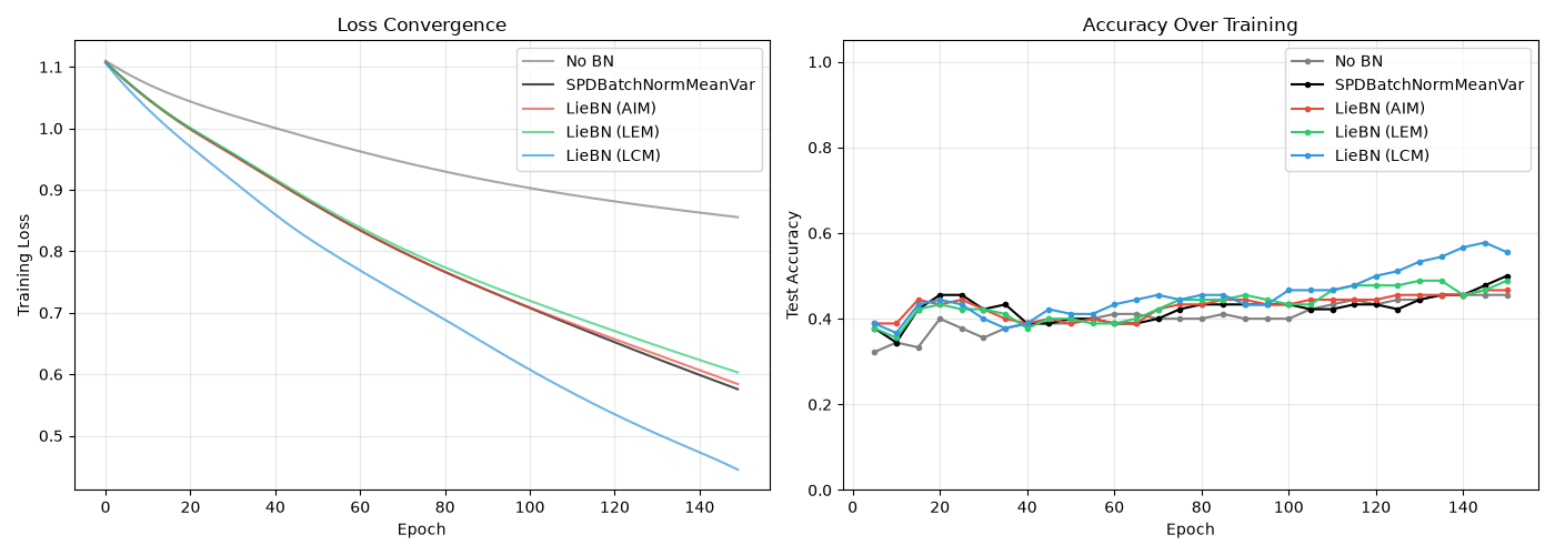
Notice the improvement! Batch normalization stabilizes the loss trajectory and allows the network to converge to a better solution.
Lie Group Batch Normalization#
SPDBatchNormLie [Chen et al., 2024]
exploits the Lie group structure of \(\spd\). Unlike
SPDBatchNormMeanVar which only supports AIRM, LieBN supports three
Riemannian metrics:
AIM (Affine-Invariant Metric): Iterative Karcher mean, full affine invariance.
LEM (Log-Euclidean Metric): Closed-form mean, fast computation.
LCM (Log-Cholesky Metric): Cholesky-based, numerically stable.
Let’s try all three:
liebn_results = {}
for metric in ["AIM", "LEM", "LCM"]:
    torch.manual_seed(42)
    model = SimpleSPDNet(8, 4, 3, bn=SPDBatchNormLie(4, metric=metric))
    losses, accs = train_model(model, X_train, y_train, X_test, y_test)
    liebn_results[metric] = (losses, accs)
    print(f"LieBN ({metric}): final accuracy = {accs[-1][1]:.1%}")
LieBN (AIM): final accuracy = 46.7%
LieBN (LEM): final accuracy = 48.9%
LieBN (LCM): final accuracy = 55.6%
Comparing Training Dynamics#
Let’s visualize how each normalization strategy affects convergence.
fig, (ax1, ax2) = plt.subplots(1, 2, figsize=(14, 5))

# Loss curves
ax1.plot(losses_none, label="No BN", alpha=0.7, color="gray")
ax1.plot(losses_rbn, label="SPDBatchNormMeanVar", alpha=0.7, color="black")
colors = {"AIM": "#e74c3c", "LEM": "#2ecc71", "LCM": "#3498db"}
for metric, (losses, _) in liebn_results.items():
    ax1.plot(losses, label=f"LieBN ({metric})", alpha=0.7, color=colors[metric])
ax1.set_xlabel("Epoch")
ax1.set_ylabel("Training Loss")
ax1.set_title("Loss Convergence")
ax1.legend()
ax1.grid(True, alpha=0.3)

# Accuracy curves
for label, accs, color in [
    ("No BN", accs_none, "gray"),
    ("SPDBatchNormMeanVar", accs_rbn, "black"),
]:
    epochs, vals = zip(*accs)
    ax2.plot(epochs, vals, "o-", label=label, color=color, markersize=3)
for metric, (_, accs) in liebn_results.items():
    epochs, vals = zip(*accs)
    ax2.plot(
        epochs,
        vals,
        "o-",
        label=f"LieBN ({metric})",
        color=colors[metric],
        markersize=3,
    )
ax2.set_xlabel("Epoch")
ax2.set_ylabel("Test Accuracy")
ax2.set_title("Accuracy Over Training")
ax2.legend()
ax2.grid(True, alpha=0.3)
ax2.set_ylim(0, 1.05)

plt.tight_layout()
plt.show()
Inspecting the LieBN Pipeline#
LieBN normalizes SPD matrices through five geometric steps:
Deformation – map SPD matrices to a codomain via the chosen metric (e.g., matrix log for LEM, Cholesky + log-diag for LCM)
Centering – translate the batch to zero/identity mean
Scaling – normalize variance by a learnable dispersion parameter
Biasing – translate by a learnable location parameter
Inverse Deformation – map back to the SPD manifold
The three metrics differ in how they perform deformation and centering:
Metric |
Deformation |
Mean |
Group Action |
|---|---|---|---|
LEM |
\(\log(X)\) |
Euclidean (closed-form) |
Additive |
LCM |
Cholesky + log-diag |
Euclidean (closed-form) |
Additive |
AIM |
\(X^\theta\) |
Karcher (iterative) |
Cholesky congruence |
Let’s watch the running variance converge during training:
torch.manual_seed(42)
A = torch.randn(64, 8, 8)
X_demo = A @ A.mT + 0.1 * torch.eye(8)

fig, ax = plt.subplots(figsize=(8, 4))
for metric in ["AIM", "LEM", "LCM"]:
    bn = SPDBatchNormLie(8, metric=metric, momentum=0.1)
    bn.train()
    variances = []
    for epoch in range(50):
        perm = torch.randperm(len(X_demo))
        for i in range(0, len(X_demo), 16):
            batch = X_demo[perm[i : i + 16]]
            if batch.shape[0] < 2:
                continue
            _ = bn(batch)
        variances.append(bn.running_var.item())
    ax.plot(variances, label=metric, color=colors[metric])

ax.set_xlabel("Epoch")
ax.set_ylabel("Running Variance")
ax.set_title("Running Variance Convergence Across Metrics")
ax.legend()
ax.grid(True, alpha=0.3)
plt.tight_layout()
plt.show()
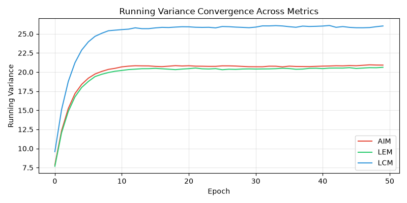
Notice that all three metrics converge, but LEM and LCM converge faster thanks to their closed-form mean computation.
Verifying SPD Output and Gradient Flow#
A critical property: batch normalization must produce valid SPD output with flowing gradients. Let’s verify:
torch.manual_seed(42)
A = torch.randn(8, 4, 4)
X_check = (A @ A.mT + 0.1 * torch.eye(4)).requires_grad_(True)

for metric in ["AIM", "LEM", "LCM"]:
    bn = SPDBatchNormLie(4, metric=metric)
    bn.train()
    out = bn(X_check)
    loss = (out * out).sum()
    loss.backward()
    eigvals = torch.linalg.eigvalsh(out.detach())
    print(
        f"{metric}: min_eigval={eigvals.min():.2e}, grad_norm={X_check.grad.norm():.4f}"
    )
    X_check.grad = None
AIM: min_eigval=3.90e-01, grad_norm=4.3125
LEM: min_eigval=3.75e-01, grad_norm=5.8443
LCM: min_eigval=2.54e-01, grad_norm=17.6761
All eigenvalues are positive (valid SPD) and gradients flow correctly through the normalization layer.
Summary#
In this tutorial you learned:
Why: Batch normalization stabilizes SPDNet training by normalizing the distribution of SPD activations
How: Riemannian BN uses the Frechet mean and variance; Lie group BN generalizes this to multiple metrics
Which metric: LEM for speed, AIM for invariance, LCM for Cholesky stability
Next steps:
See also
How to Add Batch Normalization to an SPDNet – Add BN to an existing pipeline
How to Choose a Metric for Batch Normalization – Decision guide for metric selection
Reproducing LieBN Paper Results (Table 4) – Full benchmark reproduction across HDM05, Radar, and AFEW datasets
SPDBatchNormLie– API referenceSPDBatchNormMeanVar– API reference
References#
Ziheng Chen, Yue Song, Yunmei Xu, and Nicu Sebe. A lie group approach to riemannian batch normalization. In International Conference on Learning Representations. 2024. URL: https://openreview.net/forum?id=okYdj8Ysru.
Total running time of the script: (0 minutes 13.930 seconds)
