
Note
Go to the end to download the full example code.
Learnable Wavelets with GREEN for EEG Classification#
This tutorial demonstrates how to use the GREEN (Gabor Riemann EEGNet) model for EEG classification. GREEN combines learnable Gabor wavelets with Riemannian geometry for biomarker exploration.
Introduction#
GREEN [Paillard et al., 2025] is a lightweight architecture that learns optimal time-frequency representations directly from EEG data. Unlike traditional approaches that use fixed filter banks, GREEN employs parametrized Gabor wavelets with learnable center frequencies and bandwidths.
Key features of GREEN:
Learnable wavelets: Center frequencies and FWHM are optimized during training
Riemannian geometry: SPD covariance matrices with BiMap and LogEig layers
Lightweight: Efficient architecture suitable for clinical applications
Setup and Imports#
First, we import the necessary libraries.
import warnings

import matplotlib.pyplot as plt
import numpy as np
import torch

from braindecode import EEGClassifier
from moabb.datasets import BNCI2014_001
from moabb.paradigms import MotorImagery
from sklearn.metrics import accuracy_score, balanced_accuracy_score
from sklearn.preprocessing import LabelEncoder
from skorch.callbacks import EpochScoring
from skorch.dataset import ValidSplit

from spd_learn.models import Green


warnings.filterwarnings("ignore")
Loading the Dataset#
We use the BCI Competition IV Dataset 2a (BNCI2014_001), which contains motor imagery EEG recordings from 9 subjects.
dataset = BNCI2014_001()
paradigm = MotorImagery(n_classes=4)

print(f"Dataset: {dataset.code}")
print(f"Subjects: {dataset.subject_list}")
Choosing from all possible events
Dataset: BNCI2014-001
Subjects: [1, 2, 3, 4, 5, 6, 7, 8, 9]
Creating the GREEN Model#
GREEN processes EEG through the following stages:
Wavelet Convolution: Learnable Gabor wavelets extract time-frequency features
Covariance Pooling: Compute SPD covariance matrices
Shrinkage: Ledoit-Wolf regularization for stable covariance estimation
BiMap Layers: Optional spatial filtering on the SPD manifold
LogEig + BatchReNorm: Project to tangent space with normalization
MLP Head: Classification with dropout
Key parameters:
n_freqs_init: Number of wavelet center frequencies (default: 10)kernel_width_s: Wavelet kernel width in secondsoct_min/oct_max: Frequency range in octaves (relative to 1 Hz)shrinkage_init: Initial shrinkage coefficient (sigmoid input)
# Model hyperparameters
n_chans = 22
n_outputs = 4
sfreq = 250  # Sampling frequency of BNCI2014_001

# Create GREEN model
model = Green(
    n_outputs=n_outputs,
    n_chans=n_chans,
    sfreq=sfreq,
    n_freqs_init=10,  # Number of learnable wavelets
    kernel_width_s=0.5,  # 500ms wavelet width
    oct_min=0,  # ~1 Hz minimum
    oct_max=5,  # ~32 Hz maximum (2^5)
    shrinkage_init=-3.0,  # Initial shrinkage (sigmoid(-3) ≈ 0.05)
    hidden_dim=(16,),  # Hidden layer in MLP head
    dropout=0.5,
)

print("\nGREEN Model Architecture:")
print(model)
GREEN Model Architecture:
Green(
  (conv_layers): Sequential(
    (0): WaveletConv()
  )
  (cov_layer): CovLayer()
  (spd_layers): Sequential(
    (0): Shrinkage()
  )
  (proj): Sequential(
    (0): LogEig()
    (1): BatchReNorm()
  )
  (head): Sequential(
    (0): BatchNorm1d(2530, eps=1e-05, momentum=0.1, affine=True, bias=True, track_running_stats=True)
    (1): Dropout(p=0.5, inplace=False)
    (2): Linear(in_features=2530, out_features=16, bias=True)
    (3): GELU(approximate='none')
    (4): BatchNorm1d(16, eps=1e-05, momentum=0.1, affine=True, bias=True, track_running_stats=True)
    (5): Dropout(p=0.5, inplace=False)
    (6): Linear(in_features=16, out_features=4, bias=True)
  )
)
Setting up the Classifier#
We use Braindecode’s EEGClassifier wrapper for scikit-learn compatibility.
# Training hyperparameters
batch_size = 32
max_epochs = 50
learning_rate = 1e-3

device = "cuda" if torch.cuda.is_available() else "cpu"
print(f"\nUsing device: {device}")

clf = EEGClassifier(
    model,
    criterion=torch.nn.CrossEntropyLoss,
    optimizer=torch.optim.AdamW,
    optimizer__lr=learning_rate,
    optimizer__weight_decay=1e-4,
    train_split=ValidSplit(0.1, stratified=True, random_state=42),
    batch_size=batch_size,
    max_epochs=max_epochs,
    callbacks=[
        (
            "train_acc",
            EpochScoring(
                "accuracy", lower_is_better=False, on_train=True, name="train_acc"
            ),
        ),
        (
            "bal_acc",
            EpochScoring(
                "balanced_accuracy",
                lower_is_better=False,
                on_train=False,
                name="bal_acc",
            ),
        ),
    ],
    device=device,
    verbose=1,
)
Using device: cpu
Training and Evaluation#
We train on a single subject for demonstration.
subject_id = 1

# Cache configuration
cache_config = dict(
    save_raw=True,
    save_epochs=True,
    save_array=True,
    use=True,
    overwrite_raw=False,
    overwrite_epochs=False,
    overwrite_array=False,
)

# Load data
X, labels, meta = paradigm.get_data(
    dataset=dataset, subjects=[subject_id], cache_config=cache_config
)

# Encode labels
le = LabelEncoder()
y = le.fit_transform(labels)

print(f"\nData shape: {X.shape}")
print(f"Classes: {le.classes_}")

# Split by session
train_idx = meta.query("session == '0train'").index.to_numpy()
test_idx = meta.query("session == '1test'").index.to_numpy()

print(f"Training samples: {len(train_idx)}")
print(f"Test samples: {len(test_idx)}")

# Train
clf.fit(X[train_idx], y[train_idx])

# Evaluate
y_pred_train = clf.predict(X[train_idx])
y_pred_test = clf.predict(X[test_idx])

train_acc = accuracy_score(y[train_idx], y_pred_train)
test_acc = accuracy_score(y[test_idx], y_pred_test)
test_bal_acc = balanced_accuracy_score(y[test_idx], y_pred_test)

print(f"\n{'=' * 50}")
print(f"Results for Subject {subject_id}")
print(f"{'=' * 50}")
print(f"Train Accuracy:    {train_acc * 100:.2f}%")
print(f"Test Accuracy:     {test_acc * 100:.2f}%")
print(f"Test Balanced Acc: {test_bal_acc * 100:.2f}%")
Data shape: (576, 22, 1001)
Classes: ['feet' 'left_hand' 'right_hand' 'tongue']
Training samples: 288
Test samples: 288
  epoch    bal_acc    train_acc    train_loss    valid_acc    valid_loss     dur
-------  ---------  -----------  ------------  -----------  ------------  ------
      1     0.4286       0.3438        1.3549       0.4483        1.2873  4.0886
      2     0.5402       0.6406        0.9441       0.5517        1.1893  3.7026
      3     0.6786       0.6641        0.9080       0.6897        1.1037  3.6409
      4     0.6786       0.7891        0.7796       0.6897        0.9994  3.4757
      5     0.7143       0.8086        0.7311       0.7241        0.9066  3.3601
      6     0.5491       0.8047        0.6760       0.5517        0.8626  3.0112
      7     0.6786       0.8555        0.5850       0.6897        0.8127  3.9655
      8     0.7545       0.8594        0.5566       0.7586        0.6991  4.0657
      9     0.7500       0.9180        0.4980       0.7586        0.6625  4.0458
     10     0.7500       0.8828        0.5333       0.7586        0.6716  3.3284
     11     0.7143       0.9453        0.4577       0.7241        0.6891  3.4749
     12     0.7589       0.9336        0.3986       0.7586        0.6073  3.7804
     13     0.6429       0.9102        0.4082       0.6552        0.6980  4.1337
     14     0.7188       0.9492        0.3848       0.7241        0.6201  3.6814
     15     0.7545       0.9297        0.3647       0.7586        0.5759  3.3270
     16     0.7545       0.9414        0.3518       0.7586        0.5633  4.1620
     17     0.7545       0.9492        0.3614       0.7586        0.5938  4.3153
     18     0.7634       0.9375        0.3261       0.7586        0.6017  4.6598
     19     0.7902       0.9414        0.3010       0.7931        0.5840  4.0779
     20     0.7545       0.9609        0.2883       0.7586        0.5077  4.0452
     21     0.7321       0.9492        0.2907       0.7241        0.6022  4.0781
     22     0.8214       0.9180        0.3162       0.8276        0.4801  4.0478
     23     0.8616       0.9375        0.2938       0.8621        0.4788  4.0722
     24     0.7902       0.9609        0.2506       0.7931        0.5178  4.0554
     25     0.8304       0.9688        0.2323       0.8276        0.4652  4.0480
     26     0.8973       0.9492        0.2556       0.8966        0.4255  4.0353
     27     0.8616       0.9688        0.2293       0.8621        0.4642  4.0440
     28     0.8259       0.9648        0.2219       0.8276        0.4669  3.9824
     29     0.8259       0.9727        0.2278       0.8276        0.4895  4.0385
     30     0.8259       0.9648        0.2190       0.8276        0.4341  4.0924
     31     0.7902       0.9492        0.2286       0.7931        0.4975  3.9534
     32     0.7902       0.9688        0.1934       0.7931        0.4943  4.4397
     33     0.7188       0.9609        0.2012       0.7241        0.5526  3.9508
     34     0.8616       0.9531        0.2031       0.8621        0.4780  3.9828
     35     0.8304       0.9609        0.1851       0.8276        0.4556  3.9881
     36     0.8616       0.9805        0.1694       0.8621        0.4365  4.0199
     37     0.7902       0.9414        0.1912       0.7931        0.5068  3.8805
     38     0.8616       0.9727        0.1635       0.8621        0.5142  4.0806
     39     0.8616       0.9805        0.1506       0.8621        0.5017  4.0678
     40     0.8259       0.9648        0.1497       0.8276        0.4786  4.0831
     41     0.8616       0.9844        0.1344       0.8621        0.4506  3.5876
     42     0.7902       0.9688        0.1467       0.7931        0.4484  2.9967
     43     0.7946       0.9805        0.1142       0.7931        0.5230  2.6933
     44     0.7902       0.9727        0.1393       0.7931        0.5444  2.6886
     45     0.7902       0.9688        0.1589       0.7931        0.4716  2.6929
     46     0.7902       0.9688        0.1614       0.7931        0.4449  2.7002
     47     0.6830       0.9766        0.1445       0.6897        0.5927  2.6897
     48     0.8259       0.9844        0.1364       0.8276        0.4573  2.6919
     49     0.8616       0.9805        0.1221       0.8621        0.4710  2.7518
     50     0.8304       0.9609        0.1483       0.8276        0.5344  2.6874

==================================================
Results for Subject 1
==================================================
Train Accuracy:    98.26%
Test Accuracy:     78.47%
Test Balanced Acc: 78.47%
Visualizing Learned Wavelets#
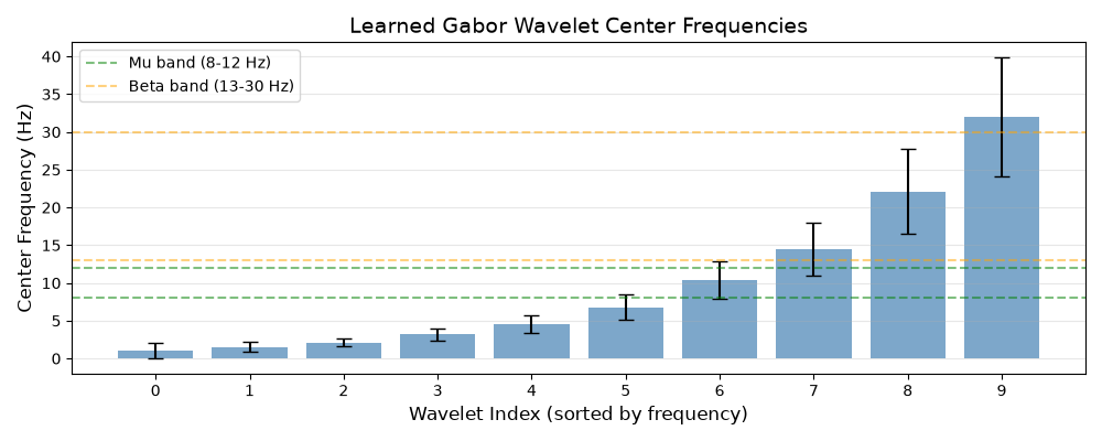
One advantage of GREEN is that we can inspect the learned wavelet parameters to understand which frequencies are most discriminative.
# Extract learned wavelet parameters
wavelet_conv = model.conv_layers[0]
foi_learned = wavelet_conv.foi.detach().cpu().numpy()  # Center frequencies (octaves)
fwhm_learned = wavelet_conv.fwhm.detach().cpu().numpy()  # Bandwidth (octaves)

# Convert from octaves to Hz
foi_hz = 2**foi_learned
bandwidth_hz = 2 ** np.abs(fwhm_learned)

print("\nLearned Wavelet Parameters:")
print("-" * 40)
for i, (f, bw) in enumerate(zip(foi_hz, bandwidth_hz)):
    print(f"Wavelet {i + 1}: Center = {f:.1f} Hz, Bandwidth = {bw:.1f} Hz")

# Plot wavelet frequencies
fig, ax = plt.subplots(figsize=(10, 4))

# Sort by center frequency for visualization
sort_idx = np.argsort(foi_hz)
foi_sorted = foi_hz[sort_idx]
bw_sorted = bandwidth_hz[sort_idx]

x_pos = np.arange(len(foi_sorted))
ax.bar(x_pos, foi_sorted, yerr=bw_sorted / 2, capsize=5, color="steelblue", alpha=0.7)
ax.set_xlabel("Wavelet Index (sorted by frequency)", fontsize=12)
ax.set_ylabel("Center Frequency (Hz)", fontsize=12)
ax.set_title("Learned Gabor Wavelet Center Frequencies", fontsize=14)
ax.set_xticks(x_pos)
ax.grid(True, alpha=0.3, axis="y")

# Add frequency band annotations
ax.axhline(y=8, color="green", linestyle="--", alpha=0.5, label="Mu band (8-12 Hz)")
ax.axhline(y=12, color="green", linestyle="--", alpha=0.5)
ax.axhline(
    y=13, color="orange", linestyle="--", alpha=0.5, label="Beta band (13-30 Hz)"
)
ax.axhline(y=30, color="orange", linestyle="--", alpha=0.5)
ax.legend(loc="upper left")

plt.tight_layout()
plt.show()
Learned Wavelet Parameters:
----------------------------------------
Wavelet 1: Center = 1.0 Hz, Bandwidth = 2.0 Hz
Wavelet 2: Center = 1.5 Hz, Bandwidth = 1.3 Hz
Wavelet 3: Center = 2.1 Hz, Bandwidth = 1.1 Hz
Wavelet 4: Center = 3.2 Hz, Bandwidth = 1.6 Hz
Wavelet 5: Center = 4.6 Hz, Bandwidth = 2.3 Hz
Wavelet 6: Center = 6.8 Hz, Bandwidth = 3.4 Hz
Wavelet 7: Center = 10.4 Hz, Bandwidth = 4.9 Hz
Wavelet 8: Center = 14.4 Hz, Bandwidth = 7.0 Hz
Wavelet 9: Center = 22.1 Hz, Bandwidth = 11.2 Hz
Wavelet 10: Center = 32.0 Hz, Bandwidth = 15.8 Hz
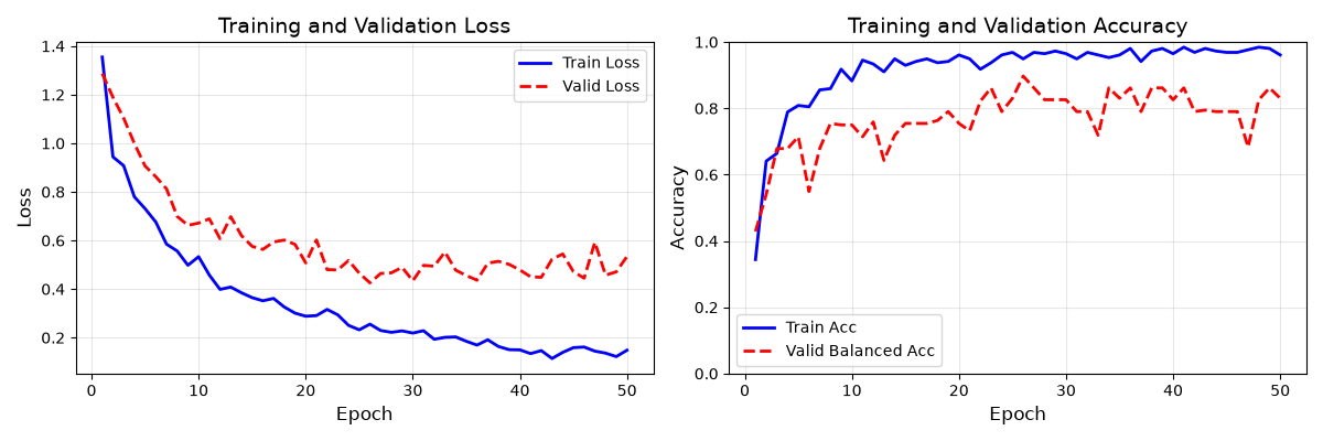
Training History#
Let’s visualize the training progress.
fig, axes = plt.subplots(1, 2, figsize=(12, 4))

history = clf.history
epochs = range(1, len(history) + 1)

# Loss
ax1 = axes[0]
ax1.plot(epochs, history[:, "train_loss"], "b-", label="Train Loss", linewidth=2)
ax1.plot(epochs, history[:, "valid_loss"], "r--", label="Valid Loss", linewidth=2)
ax1.set_xlabel("Epoch", fontsize=12)
ax1.set_ylabel("Loss", fontsize=12)
ax1.set_title("Training and Validation Loss", fontsize=14)
ax1.legend(fontsize=10)
ax1.grid(True, alpha=0.3)

# Accuracy
ax2 = axes[1]
ax2.plot(epochs, history[:, "train_acc"], "b-", label="Train Acc", linewidth=2)
ax2.plot(epochs, history[:, "bal_acc"], "r--", label="Valid Balanced Acc", linewidth=2)
ax2.set_xlabel("Epoch", fontsize=12)
ax2.set_ylabel("Accuracy", fontsize=12)
ax2.set_title("Training and Validation Accuracy", fontsize=14)
ax2.legend(fontsize=10)
ax2.grid(True, alpha=0.3)
ax2.set_ylim([0, 1])

plt.tight_layout()
plt.show()
Summary#
In this tutorial, we demonstrated how to:
Create a GREEN model with learnable Gabor wavelets
Train and evaluate on motor imagery EEG data
Visualize the learned wavelet parameters
GREEN’s learnable wavelets allow the model to discover optimal time-frequency representations for the classification task, often focusing on the mu (8-12 Hz) and beta (13-30 Hz) rhythms known to be modulated during motor imagery.
Total running time of the script: (3 minutes 8.270 seconds)
