Understanding Symmetric Positive Definite (SPD) Matrices

This tutorial provides a comprehensive introduction to Symmetric Positive Definite (SPD) matrices and explains why Riemannian geometry is essential for working with them in machine learning.

What are SPD Matrices?

A Symmetric Positive Definite (SPD) matrix is a square matrix \(S\) that satisfies two properties:

1. Symmetry: \(S = S^T\)

2. Positive Definiteness: \(x^T S x > 0\) for all non-zero vectors \(x\)

Equivalently, an SPD matrix has all positive eigenvalues.

SPD matrices appear naturally in many applications:

• Covariance matrices in statistics and signal processing

• Diffusion tensors in medical imaging (DTI)

• Kernels in machine learning (Gram matrices)

• Inertia tensors in physics

Setup and Imports

import matplotlib.pyplot as plt
import numpy as np
import torch

from spd_learn.functional import (
    log_euclidean_distance,
    log_euclidean_mean,
    matrix_exp,
    matrix_log,
)


# Set random seeds for reproducibility
np.random.seed(42)
torch.manual_seed(42)

<torch._C.Generator object at 0x7f32c5b2e770>

Creating SPD Matrices

There are several ways to create SPD matrices. The most common is through a product \(A A^T\) where \(A\) has full rank.

def create_spd_matrix(n, eigenvalues=None, dtype=torch.float64):
    """Create an SPD matrix with given eigenvalues.

    Parameters
    ----------
    n : int
        Matrix dimension.
    eigenvalues : array-like, optional
        Desired eigenvalues. If None, random positive values are used.
    dtype : torch.dtype
        Data type for the tensor.

    Returns
    -------
    torch.Tensor
        An n x n SPD matrix.
    """
    # Random orthogonal matrix via QR decomposition
    Q, _ = torch.linalg.qr(torch.randn(n, n, dtype=dtype))

    if eigenvalues is None:
        eigenvalues = torch.abs(torch.randn(n, dtype=dtype)) + 0.5  # Ensure positive
    else:
        eigenvalues = torch.tensor(eigenvalues, dtype=dtype)

    return Q @ torch.diag(eigenvalues) @ Q.T


# Create a simple 2x2 SPD matrix
A = create_spd_matrix(2, eigenvalues=[2.0, 0.5])
print("SPD Matrix A:")
print(A.numpy())
print(f"\nEigenvalues: {torch.linalg.eigvalsh(A).numpy()}")
print(f"Is symmetric: {torch.allclose(A, A.T)}")
print(f"All eigenvalues positive: {torch.all(torch.linalg.eigvalsh(A) > 0).item()}")

SPD Matrix A:
[[1.51014416 0.703438  ]
 [0.703438   0.98985584]]

Eigenvalues: [0.5 2. ]
Is symmetric: True
All eigenvalues positive: True

Visualizing 2x2 SPD Matrices as Ellipses

A 2x2 SPD matrix can be visualized as an ellipse. The matrix \(S\) defines an ellipse as the set of points satisfying:

\[\{x : x^T S^{-1} x = 1\}\]

The eigenvectors give the principal axes, and the square roots of eigenvalues give the semi-axis lengths.

def spd_to_ellipse(spd_matrix, n_points=100):
    """Convert 2x2 SPD matrix to ellipse coordinates."""
    eigvals, eigvecs = np.linalg.eigh(spd_matrix)

    # Parametric ellipse
    theta = np.linspace(0, 2 * np.pi, n_points)
    circle = np.array([np.cos(theta), np.sin(theta)])

    # Transform circle to ellipse
    transform = eigvecs @ np.diag(np.sqrt(eigvals))
    ellipse = transform @ circle

    return ellipse[0], ellipse[1]


# Create two SPD matrices with different properties
S1 = create_spd_matrix(2, eigenvalues=[3.0, 1.0])
S2 = create_spd_matrix(2, eigenvalues=[2.0, 2.0])
S3 = create_spd_matrix(2, eigenvalues=[4.0, 0.5])

fig, axes = plt.subplots(1, 3, figsize=(12, 4))

for ax, S, title in zip(
    axes,
    [S1, S2, S3],
    ["Anisotropic (3, 1)", "Isotropic (2, 2)", "Highly Anisotropic (4, 0.5)"],
):
    # Convert to numpy for plotting
    S_np = S.numpy()
    x, y = spd_to_ellipse(S_np)
    ax.fill(x, y, alpha=0.3, color="blue")
    ax.plot(x, y, "b-", linewidth=2)

    # Draw eigenvalue axes
    eigvals, eigvecs = np.linalg.eigh(S_np)
    for i in range(2):
        vec = eigvecs[:, i] * np.sqrt(eigvals[i])
        ax.arrow(0, 0, vec[0], vec[1], head_width=0.1, color="red", linewidth=2)

    ax.set_xlim(-3, 3)
    ax.set_ylim(-3, 3)
    ax.set_aspect("equal")
    ax.grid(True, alpha=0.3)
    ax.set_title(title, fontsize=11)
    ax.axhline(y=0, color="k", linewidth=0.5)
    ax.axvline(x=0, color="k", linewidth=0.5)

plt.suptitle("SPD Matrices Visualized as Ellipses", fontsize=14, fontweight="bold")
plt.tight_layout()
plt.show()

Why SPD Matrices Do Not Form a Vector Space

A critical insight is that SPD matrices do NOT form a vector space. The set of SPD matrices, denoted \(\mathcal{S}_{++}^n\), is not closed under standard linear operations:

1. Scalar multiplication: \(-1 \cdot S\) is not SPD

2. Addition boundary: Sum of SPD matrices is SPD, but differences may not be

More importantly, the Euclidean mean of SPD matrices exhibits problematic behavior known as the “swelling effect.”

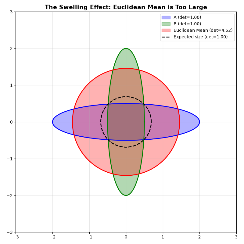
The Swelling Effect

When we compute the arithmetic (Euclidean) mean of SPD matrices, the determinant of the mean is often larger than the geometric mean of the individual determinants. This violates the intuition that an “average” should be “in the middle.”

def euclidean_mean(matrices):
    """Compute the arithmetic mean of matrices."""
    return torch.mean(torch.stack(matrices), dim=0)


def geometric_mean_det(matrices):
    """Compute geometric mean of determinants."""
    dets = torch.stack([torch.linalg.det(m) for m in matrices])
    return torch.exp(torch.mean(torch.log(dets)))


# Create two very different SPD matrices
A = torch.tensor(
    [[4.0, 0.0], [0.0, 0.25]], dtype=torch.float64
)  # Large in x, small in y
B = torch.tensor(
    [[0.25, 0.0], [0.0, 4.0]], dtype=torch.float64
)  # Small in x, large in y

# Compute means
mean_euclidean = euclidean_mean([A, B])
det_A = torch.linalg.det(A)
det_B = torch.linalg.det(B)
det_mean = torch.linalg.det(mean_euclidean)
geo_mean_det = geometric_mean_det([A, B])

print("Matrix A:")
print(A.numpy())
print(f"det(A) = {det_A.item():.3f}")
print("\nMatrix B:")
print(B.numpy())
print(f"det(B) = {det_B.item():.3f}")
print("\nEuclidean Mean:")
print(mean_euclidean.numpy())
print(f"det(Mean) = {det_mean.item():.3f}")
print(f"\nGeometric mean of determinants: {geo_mean_det.item():.3f}")
print(
    f"\nSwelling ratio: det(Mean) / geo_mean = {(det_mean / geo_mean_det).item():.3f}"
)

Matrix A:
[[4.   0.  ]
 [0.   0.25]]
det(A) = 1.000

Matrix B:
[[0.25 0.  ]
 [0.   4.  ]]
det(B) = 1.000

Euclidean Mean:
[[2.125 0.   ]
 [0.    2.125]]
det(Mean) = 4.516

Geometric mean of determinants: 1.000

Swelling ratio: det(Mean) / geo_mean = 4.516

Visualizing the Swelling Effect

The Euclidean mean produces an ellipse that is “swollen” - its area (proportional to det) is larger than expected.

fig, ax = plt.subplots(1, 1, figsize=(8, 8))

# Convert to numpy for plotting
A_np, B_np = A.numpy(), B.numpy()
mean_euclidean_np = mean_euclidean.numpy()

# Plot original matrices
x_A, y_A = spd_to_ellipse(A_np)
x_B, y_B = spd_to_ellipse(B_np)
x_mean, y_mean = spd_to_ellipse(mean_euclidean_np)

ax.fill(x_A, y_A, alpha=0.3, color="blue", label=f"A (det={det_A.item():.2f})")
ax.plot(x_A, y_A, "b-", linewidth=2)

ax.fill(x_B, y_B, alpha=0.3, color="green", label=f"B (det={det_B.item():.2f})")
ax.plot(x_B, y_B, "g-", linewidth=2)

ax.fill(
    x_mean,
    y_mean,
    alpha=0.3,
    color="red",
    label=f"Euclidean Mean (det={det_mean.item():.2f})",
)
ax.plot(x_mean, y_mean, "r-", linewidth=2)

# Reference: what the "ideal" mean should look like (same determinant as geometric mean)
ideal_scale = np.sqrt(geo_mean_det.item() / det_mean.item())
ax.plot(
    x_mean * ideal_scale,
    y_mean * ideal_scale,
    "k--",
    linewidth=2,
    label=f"Expected size (det={geo_mean_det.item():.2f})",
)

ax.set_xlim(-3, 3)
ax.set_ylim(-3, 3)
ax.set_aspect("equal")
ax.grid(True, alpha=0.3)
ax.legend(loc="upper right", fontsize=10)
ax.set_title(
    "The Swelling Effect: Euclidean Mean is Too Large",
    fontsize=14,
    fontweight="bold",
)
plt.tight_layout()
plt.show()

The SPD Manifold: A Cone Structure

The set of SPD matrices forms an open convex cone in the space of symmetric matrices. We can visualize this for 2x2 matrices:

A 2x2 symmetric matrix has 3 unique elements: \([a, b, c]\) where

\[\begin{split}S = \begin{pmatrix} a & b \\ b & c \end{pmatrix}\end{split}\]

The SPD condition requires:

• \(a > 0\) (first diagonal positive)

• \(c > 0\) (second diagonal positive)

• \(ac - b^2 > 0\) (positive determinant)

This defines a cone in 3D space.

def is_spd_2x2(a, b, c):
    """Check if 2x2 symmetric matrix [[a,b],[b,c]] is SPD."""
    return (a > 0) & (c > 0) & (a * c - b**2 > 0)


# Create a grid
a_vals = np.linspace(0.1, 3, 30)
b_vals = np.linspace(-2, 2, 30)
c_vals = np.linspace(0.1, 3, 30)

# Visualize the cone boundary (det = 0 surface)
fig = plt.figure(figsize=(10, 8))
ax = fig.add_subplot(111, projection="3d")

# Create mesh for b vs sqrt(ac)
A_mesh, C_mesh = np.meshgrid(a_vals, c_vals)
# Boundary: b^2 = ac, so b = +/- sqrt(ac)
B_boundary = np.sqrt(A_mesh * C_mesh)

# Plot the cone boundary
ax.plot_surface(
    A_mesh, B_boundary, C_mesh, alpha=0.3, color="blue", label="Boundary (det=0)"
)
ax.plot_surface(A_mesh, -B_boundary, C_mesh, alpha=0.3, color="blue")

# Plot some SPD points inside the cone
n_points = 50
spd_points = []
for _ in range(n_points):
    a = np.random.uniform(0.5, 2.5)
    c = np.random.uniform(0.5, 2.5)
    b_max = np.sqrt(a * c) * 0.9  # Inside the cone
    b = np.random.uniform(-b_max, b_max)
    spd_points.append([a, b, c])

spd_points = np.array(spd_points)
ax.scatter(
    spd_points[:, 0],
    spd_points[:, 1],
    spd_points[:, 2],
    c="red",
    s=20,
    label="SPD matrices",
)

ax.set_xlabel("a (diagonal)", fontsize=10)
ax.set_ylabel("b (off-diagonal)", fontsize=10)
ax.set_zlabel("c (diagonal)", fontsize=10)
ax.set_title(
    "SPD Manifold as a Cone in 3D\n(2x2 symmetric matrices)",
    fontsize=14,
    fontweight="bold",
)
plt.tight_layout()
plt.show()

Why Riemannian Geometry?

Since SPD matrices do not form a vector space, we need a different framework for computing distances and means. Riemannian geometry [Pennec et al., 2006] provides this framework by:

1. Defining a metric (inner product) at each point on the manifold

2. Using geodesics (shortest paths) instead of straight lines

3. Computing exponential/logarithmic maps to move between the manifold and tangent spaces

The most common metrics for SPD matrices are:

• Affine Invariant Riemannian Metric (AIRM)

• Log-Euclidean Metric

We focus on the Log-Euclidean metric as it is computationally efficient.

Matrix Logarithm and Exponential

The matrix logarithm maps an SPD matrix to a symmetric matrix (the tangent space at the identity). For SPD matrix \(S\) with eigendecomposition \(S = U \Lambda U^T\):

\[\log(S) = U \log(\Lambda) U^T\]

The matrix exponential is the inverse operation:

\[\exp(X) = U \exp(\Lambda) U^T\]

These operations are key to the Log-Euclidean framework.

# Create an SPD matrix
S = torch.tensor([[2.0, 0.5], [0.5, 1.0]], dtype=torch.float64)

print("Original SPD Matrix S:")
print(S.numpy())
print(f"Eigenvalues: {torch.linalg.eigvalsh(S).numpy()}")

# Compute matrix logarithm
log_S = matrix_log.apply(S)
print("\nMatrix Logarithm log(S):")
print(log_S.numpy())
print(f"Eigenvalues of log(S): {torch.linalg.eigvalsh(log_S).numpy()}")

# Verify: exp(log(S)) = S
recovered_S = matrix_exp.apply(log_S)
print("\nRecovered S = exp(log(S)):")
print(recovered_S.numpy())
print(f"Reconstruction error: {torch.norm(recovered_S - S).item():.2e}")

Original SPD Matrix S:
[[2.  0.5]
 [0.5 1. ]]
Eigenvalues: [0.79289322 2.20710678]

Matrix Logarithm log(S):
[[ 0.64175791  0.36195001]
 [ 0.36195001 -0.08214212]]
Eigenvalues of log(S): [-0.23206672  0.79168251]

Recovered S = exp(log(S)):
[[2.  0.5]
 [0.5 1. ]]
Reconstruction error: 3.33e-16

Log-Euclidean Distance

The Log-Euclidean distance [Arsigny et al., 2007] is defined as the Frobenius norm of the difference of matrix logarithms:

\[d_{LE}(A, B) = \|\log(A) - \log(B)\|_F\]

This distance respects the manifold structure better than the Euclidean distance \(\|A - B\|_F\).

# Create two SPD matrices
A = torch.tensor([[2.0, 0.3], [0.3, 1.0]], dtype=torch.float64)
B = torch.tensor([[1.5, -0.2], [-0.2, 0.8]], dtype=torch.float64)

# Euclidean distance
dist_euclidean = torch.norm(A - B, p="fro")

# Log-Euclidean distance
dist_log_euclidean = log_euclidean_distance(A, B)

print("Matrix A:")
print(A.numpy())
print("\nMatrix B:")
print(B.numpy())
print(f"\nEuclidean distance: {dist_euclidean.item():.4f}")
print(f"Log-Euclidean distance: {dist_log_euclidean.item():.4f}")

Matrix A:
[[2.  0.3]
 [0.3 1. ]]

Matrix B:
[[ 1.5 -0.2]
 [-0.2  0.8]]

Euclidean distance: 0.8888
Log-Euclidean distance: 0.6596

Log-Euclidean Mean

The Log-Euclidean mean is computed by:

1. Take the matrix logarithm of each SPD matrix

2. Compute the arithmetic mean in log-space

3. Apply the matrix exponential to return to SPD

\[\bar{S}_{LE} = \exp\left(\frac{1}{n}\sum_{i=1}^n \log(S_i)\right)\]

This mean does not suffer from the swelling effect!

# Create batch of SPD matrices
S1 = torch.tensor([[4.0, 0.0], [0.0, 0.25]], dtype=torch.float64)
S2 = torch.tensor([[0.25, 0.0], [0.0, 4.0]], dtype=torch.float64)

# Euclidean mean
mean_euclidean = (S1 + S2) / 2

# Log-Euclidean mean using weighted mean with equal weights
# Stack matrices and create uniform weights
S_stack = torch.stack([S1, S2], dim=0)  # (2, 2, 2)
weights = torch.tensor([[0.5, 0.5]], dtype=torch.float64)  # (1, 2)
mean_log_euclidean = log_euclidean_mean(weights, S_stack).squeeze(0)

print("SPD Matrix S1:")
print(S1.numpy())
print(f"det(S1) = {torch.linalg.det(S1).item():.3f}")

print("\nSPD Matrix S2:")
print(S2.numpy())
print(f"det(S2) = {torch.linalg.det(S2).item():.3f}")

print("\nEuclidean Mean:")
print(mean_euclidean.numpy())
print(f"det(Euclidean Mean) = {torch.linalg.det(mean_euclidean).item():.3f}")

print("\nLog-Euclidean Mean:")
print(mean_log_euclidean.numpy())
print(f"det(Log-Euclidean Mean) = {torch.linalg.det(mean_log_euclidean).item():.3f}")

geo_mean_det = np.sqrt(torch.linalg.det(S1).item() * torch.linalg.det(S2).item())
print(f"\nGeometric mean of determinants: {geo_mean_det:.3f}")

SPD Matrix S1:
[[4.   0.  ]
 [0.   0.25]]
det(S1) = 1.000

SPD Matrix S2:
[[0.25 0.  ]
 [0.   4.  ]]
det(S2) = 1.000

Euclidean Mean:
[[2.125 0.   ]
 [0.    2.125]]
det(Euclidean Mean) = 4.516

Log-Euclidean Mean:
[[1. 0.]
 [0. 1.]]
det(Log-Euclidean Mean) = 1.000

Geometric mean of determinants: 1.000

Comparing Euclidean vs Log-Euclidean Means

Let us visualize the difference between the two means. The Log-Euclidean mean respects the manifold geometry and does not exhibit swelling.

fig, axes = plt.subplots(1, 2, figsize=(14, 6))

# Convert torch tensors to numpy for plotting
S1_np = S1.numpy()
S2_np = S2.numpy()
mean_euc_np = mean_euclidean.numpy()
mean_le_np = mean_log_euclidean.numpy()

# Left plot: Euclidean mean
ax = axes[0]
x1, y1 = spd_to_ellipse(S1_np)
x2, y2 = spd_to_ellipse(S2_np)
x_mean_euc, y_mean_euc = spd_to_ellipse(mean_euc_np)

ax.fill(x1, y1, alpha=0.3, color="blue", label="S1")
ax.plot(x1, y1, "b-", linewidth=2)
ax.fill(x2, y2, alpha=0.3, color="green", label="S2")
ax.plot(x2, y2, "g-", linewidth=2)
ax.fill(
    x_mean_euc,
    y_mean_euc,
    alpha=0.3,
    color="red",
    label=f"Euclidean Mean (det={np.linalg.det(mean_euc_np):.2f})",
)
ax.plot(x_mean_euc, y_mean_euc, "r-", linewidth=2)

ax.set_xlim(-3, 3)
ax.set_ylim(-3, 3)
ax.set_aspect("equal")
ax.grid(True, alpha=0.3)
ax.legend(loc="upper right", fontsize=9)
ax.set_title("Euclidean Mean\n(Swelling Effect)", fontsize=12, fontweight="bold")

# Right plot: Log-Euclidean mean
ax = axes[1]
x_mean_le, y_mean_le = spd_to_ellipse(mean_le_np)

ax.fill(x1, y1, alpha=0.3, color="blue", label="S1")
ax.plot(x1, y1, "b-", linewidth=2)
ax.fill(x2, y2, alpha=0.3, color="green", label="S2")
ax.plot(x2, y2, "g-", linewidth=2)
ax.fill(
    x_mean_le,
    y_mean_le,
    alpha=0.3,
    color="purple",
    label=f"Log-Euclidean Mean (det={np.linalg.det(mean_le_np):.2f})",
)
ax.plot(x_mean_le, y_mean_le, "m-", linewidth=2)

ax.set_xlim(-3, 3)
ax.set_ylim(-3, 3)
ax.set_aspect("equal")
ax.grid(True, alpha=0.3)
ax.legend(loc="upper right", fontsize=9)
ax.set_title(
    "Log-Euclidean Mean\n(Respects Manifold Geometry)",
    fontsize=12,
    fontweight="bold",
)

plt.suptitle(
    "Comparison of Mean Computation Methods",
    fontsize=14,
    fontweight="bold",
    y=1.02,
)
plt.tight_layout()
plt.show()

Interpolation: Euclidean vs Geodesic

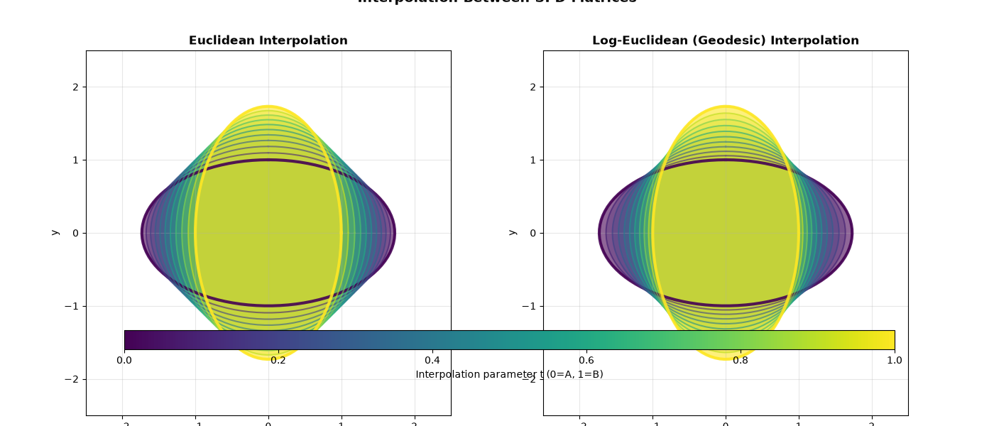
Another key difference is in interpolation. Euclidean interpolation (straight line) may produce matrices that are “far” from both endpoints in the manifold sense. Geodesic interpolation follows the shortest path on the manifold.

def interpolate_euclidean(A, B, t):
    """Linear interpolation: (1-t)*A + t*B"""
    return (1 - t) * A + t * B


def interpolate_log_euclidean(A, B, t):
    """Log-Euclidean interpolation."""
    log_A = matrix_log.apply(A)
    log_B = matrix_log.apply(B)
    log_interp = (1 - t) * log_A + t * log_B
    return matrix_exp.apply(log_interp)


# Create two SPD matrices
A = torch.tensor([[3.0, 0.0], [0.0, 1.0]], dtype=torch.float64)
B = torch.tensor([[1.0, 0.0], [0.0, 3.0]], dtype=torch.float64)

# Interpolation steps
t_values = np.linspace(0, 1, 11)

fig, axes = plt.subplots(1, 2, figsize=(14, 6))

# Colors for interpolation
colors = plt.cm.viridis(t_values)

# Euclidean interpolation
ax = axes[0]
for t, color in zip(t_values, colors):
    interp = interpolate_euclidean(A, B, t)
    x, y = spd_to_ellipse(interp.numpy())
    alpha = 0.3 if t not in [0, 1] else 0.6
    lw = 1.5 if t not in [0, 1] else 3
    ax.plot(x, y, color=color, linewidth=lw, alpha=alpha + 0.3)
    ax.fill(x, y, color=color, alpha=alpha)

ax.set_xlim(-2.5, 2.5)
ax.set_ylim(-2.5, 2.5)
ax.set_aspect("equal")
ax.grid(True, alpha=0.3)
ax.set_title("Euclidean Interpolation", fontsize=12, fontweight="bold")
ax.set_xlabel("x", fontsize=10)
ax.set_ylabel("y", fontsize=10)

# Log-Euclidean interpolation
ax = axes[1]
for t, color in zip(t_values, colors):
    interp = interpolate_log_euclidean(A, B, t)
    x, y = spd_to_ellipse(interp.numpy())
    alpha = 0.3 if t not in [0, 1] else 0.6
    lw = 1.5 if t not in [0, 1] else 3
    ax.plot(x, y, color=color, linewidth=lw, alpha=alpha + 0.3)
    ax.fill(x, y, color=color, alpha=alpha)

ax.set_xlim(-2.5, 2.5)
ax.set_ylim(-2.5, 2.5)
ax.set_aspect("equal")
ax.grid(True, alpha=0.3)
ax.set_title("Log-Euclidean (Geodesic) Interpolation", fontsize=12, fontweight="bold")
ax.set_xlabel("x", fontsize=10)
ax.set_ylabel("y", fontsize=10)

# Add colorbar
sm = plt.cm.ScalarMappable(cmap="viridis", norm=plt.Normalize(0, 1))
sm.set_array([])
cbar = plt.colorbar(sm, ax=axes, orientation="horizontal", pad=0.1, aspect=40)
cbar.set_label("Interpolation parameter t (0=A, 1=B)", fontsize=10)

plt.suptitle(
    "Interpolation Between SPD Matrices",
    fontsize=14,
    fontweight="bold",
    y=1.02,
)
plt.tight_layout()
plt.show()

/home/runner/work/spd_learn/spd_learn/examples/tutorials/tutorial_01_spd_concepts.py:681: UserWarning: This figure includes Axes that are not compatible with tight_layout, so results might be incorrect.
  plt.tight_layout()

Determinant Along Interpolation Paths

We can further see the swelling effect by plotting the determinant along the interpolation path. The Euclidean path shows determinant increase in the middle, while the geodesic path is monotonic.

det_euclidean = []
det_geodesic = []

for t in t_values:
    interp_euc = interpolate_euclidean(A, B, t)
    interp_geo = interpolate_log_euclidean(A, B, t)
    det_euclidean.append(torch.linalg.det(interp_euc).item())
    det_geodesic.append(torch.linalg.det(interp_geo).item())

fig, ax = plt.subplots(figsize=(10, 6))

ax.plot(
    t_values, det_euclidean, "r-o", linewidth=2, markersize=8, label="Euclidean Path"
)
ax.plot(
    t_values, det_geodesic, "b-s", linewidth=2, markersize=8, label="Log-Euclidean Path"
)

# Reference line: geometric interpolation of determinants
det_geo_interp = [
    det_euclidean[0] ** (1 - t) * det_euclidean[-1] ** t for t in t_values
]
ax.plot(
    t_values,
    det_geo_interp,
    "g--",
    linewidth=2,
    label="Geometric Interpolation of det",
)

ax.axhline(y=det_euclidean[0], color="gray", linestyle=":", alpha=0.7)
ax.axhline(y=det_euclidean[-1], color="gray", linestyle=":", alpha=0.7)

ax.set_xlabel("Interpolation parameter t", fontsize=12)
ax.set_ylabel("Determinant", fontsize=12)
ax.set_title(
    "Determinant Along Interpolation Paths\n(Swelling visible in Euclidean path)",
    fontsize=14,
    fontweight="bold",
)
ax.legend(fontsize=10)
ax.grid(True, alpha=0.3)
plt.tight_layout()
plt.show()

Computing Distances in a Batch

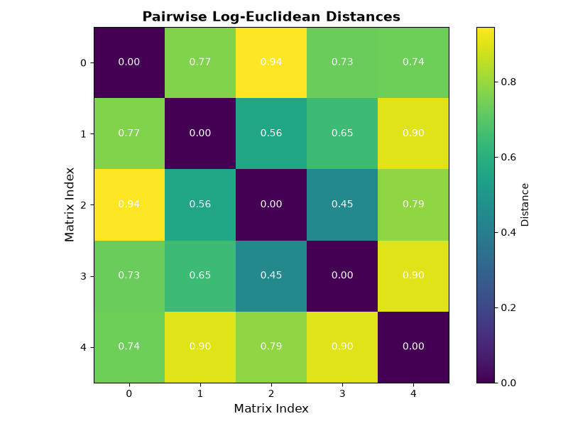
SPD Learn supports batched operations for efficient computation. Let us compute pairwise distances between multiple SPD matrices.

def generate_random_spd_batch(batch_size, n=2, dtype=torch.float64):
    """Generate batch of random SPD matrices using PyTorch."""
    matrices = []
    for _ in range(batch_size):
        Q, _ = torch.linalg.qr(torch.randn(n, n, dtype=dtype))
        eigvals = torch.abs(torch.randn(n, dtype=dtype)) + 0.5
        matrices.append(Q @ torch.diag(eigvals) @ Q.T)
    return torch.stack(matrices)


# Generate batch of SPD matrices
batch = generate_random_spd_batch(5, n=2)
print(f"Batch shape: {batch.shape}")

# Compute pairwise Log-Euclidean distances
n_matrices = batch.shape[0]
distances = torch.zeros(n_matrices, n_matrices, dtype=torch.float64)

for i in range(n_matrices):
    for j in range(n_matrices):
        distances[i, j] = log_euclidean_distance(batch[i], batch[j])

print("\nPairwise Log-Euclidean Distance Matrix:")
print(distances.numpy().round(3))

# Visualize
fig, ax = plt.subplots(figsize=(8, 6))
im = ax.imshow(distances.numpy(), cmap="viridis")
ax.set_xticks(range(n_matrices))
ax.set_yticks(range(n_matrices))
ax.set_xlabel("Matrix Index", fontsize=12)
ax.set_ylabel("Matrix Index", fontsize=12)
ax.set_title("Pairwise Log-Euclidean Distances", fontsize=14, fontweight="bold")
plt.colorbar(im, ax=ax, label="Distance")

# Add text annotations
for i in range(n_matrices):
    for j in range(n_matrices):
        text = ax.text(
            j, i, f"{distances[i, j]:.2f}", ha="center", va="center", color="white"
        )

plt.tight_layout()
plt.show()

Batch shape: torch.Size([5, 2, 2])

Pairwise Log-Euclidean Distance Matrix:
[[0.    0.767 0.945 0.729 0.738]
 [0.767 0.    0.557 0.646 0.9  ]
 [0.945 0.557 0.    0.445 0.788]
 [0.729 0.646 0.445 0.    0.898]
 [0.738 0.9   0.788 0.898 0.   ]]

Summary

In this tutorial, we learned:

1. SPD matrices are symmetric matrices with positive eigenvalues. They appear in covariance matrices, diffusion tensors, and kernels.

2. SPD matrices do not form a vector space - the Euclidean mean exhibits the “swelling effect” where the determinant is inflated.

3. The SPD manifold is a cone in the space of symmetric matrices.

4. Riemannian geometry provides proper tools for working with SPD matrices:

   • matrix_log maps SPD to symmetric (tangent space)

   • matrix_exp maps symmetric back to SPD

   • log_euclidean_distance computes manifold-respecting distance

   • log_euclidean_mean computes the geometric mean

5. Log-Euclidean operations avoid the swelling effect and respect the manifold structure.

These concepts form the foundation for deep learning on SPD manifolds [Huang and Van Gool, 2017], which is the focus of the SPD Learn library.