spd_learn.modules.ReEig

class spd_learn.modules.ReEig(threshold=None, autograd=False, device=None, dtype=None)

Bases: Module

Rectified Eigenvalue Layer (ReEig).

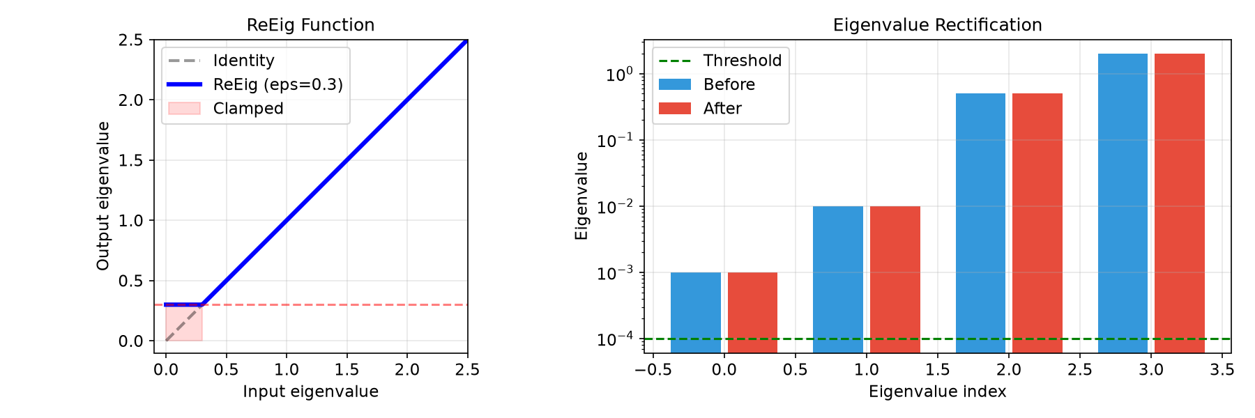
This layer rectifies eigenvalues to ensure numerical stability and maintains positive definiteness [Huang and Van Gool, 2017]. It applies a rectified linear unit (ReLU) to the eigenvalues of a symmetric matrix, introducing non-linearity while preserving the SPD property.

\[\text{ReEig}(X) = U \max(\Lambda, \varepsilon I) U^\top\]

where \(X = U \Lambda U^\top\) is the eigendecomposition and \(\varepsilon > 0\) is a rectification threshold that prevents eigenvalues from collapsing to zero.

This operation prevents eigenvalues from becoming arbitrarily small and ensures that the output remains well-conditioned on the SPD manifold, which is crucial for stable training of subsequent spectral layers (e.g., LogEig).

Parameters:

• threshold (float, optional) – The threshold for the rectified linear unit. If None, uses a dtype-aware threshold from the unified numerical configuration. Default: None.

• autograd (bool, default=False) – Whether to use the autograd backend.

Notes

When threshold=None, the actual threshold is computed at runtime based on the input tensor’s dtype using the unified numerical configuration. This ensures appropriate thresholds for different precisions (float16, float32, float64).

See also

LogEig

Projects SPD matrices to the tangent space via matrix logarithm.

BiMap

Bilinear mapping layer for dimensionality reduction.

SPDBatchNormMeanVar

Riemannian batch normalization for SPD matrices.

clamp_eigvals()

Functional version of eigenvalue clamping.

Examples

>>> import torch
>>> from spd_learn.modules import ReEig
>>> # Use default dtype-aware threshold
>>> layer = ReEig()
>>> X = torch.randn(2, 5, 5)
>>> X = X @ X.mT  # Make SPD
>>> Y = layer(X)
>>> # Use explicit threshold
>>> layer_explicit = ReEig(threshold=1e-3)

import torch
import numpy as np
import matplotlib.pyplot as plt
from spd_learn.modules import ReEig

# Visualize ReEig rectification function
fig, axes = plt.subplots(1, 2, figsize=(12, 4))

# Left: ReEig function
ax1 = axes[0]
epsilon = 0.3
x = np.linspace(0, 2.5, 200)
y_reeig = np.maximum(x, epsilon)

ax1.plot(x, x, 'k--', alpha=0.4, label='Identity', linewidth=2)
ax1.plot(x, y_reeig, 'b-', linewidth=3, label=f'ReEig (eps={epsilon})')
ax1.fill_between([0, epsilon], [epsilon, epsilon], [0, 0],
                 color='red', alpha=0.15, label='Clamped')
ax1.axhline(y=epsilon, color='red', linestyle='--', alpha=0.5)
ax1.set_xlim(-0.1, 2.5)
ax1.set_ylim(-0.1, 2.5)
ax1.set_xlabel('Input eigenvalue')
ax1.set_ylabel('Output eigenvalue')
ax1.set_title('ReEig Function')
ax1.legend()
ax1.grid(True, alpha=0.3)
ax1.set_aspect('equal')

# Right: Eigenvalue comparison
ax2 = axes[1]
torch.manual_seed(42)
eigvals = torch.tensor([2.0, 0.5, 0.01, 0.001])
eigvecs = torch.linalg.qr(torch.randn(4, 4))[0]
X = eigvecs @ torch.diag(eigvals) @ eigvecs.T
X = X.unsqueeze(0)

reeig = ReEig(threshold=1e-4)
Y = reeig(X)

ev_before = torch.linalg.eigvalsh(X[0]).numpy()
ev_after = torch.linalg.eigvalsh(Y[0]).numpy()

x_pos = np.arange(4)
ax2.bar(x_pos - 0.2, ev_before, 0.35, label='Before', color='#3498db')
ax2.bar(x_pos + 0.2, ev_after, 0.35, label='After', color='#e74c3c')
ax2.axhline(y=1e-4, color='green', linestyle='--', label='Threshold')
ax2.set_yscale('log')
ax2.set_xlabel('Eigenvalue index')
ax2.set_ylabel('Eigenvalue')
ax2.set_title('Eigenvalue Rectification')
ax2.legend()
ax2.grid(True, alpha=0.3)

plt.tight_layout()
plt.show()

(Source code)

forward(X: Tensor) → Tensor

Forward pass of the ReEig layer.

Parameters:

X (torch.Tensor) – Input symmetric matrix.

Returns:

The output matrix with rectified eigenvalues.

Return type:

torch.Tensor

threshold_: Tensor