User Guide

A practical introduction to deep learning on SPD matrices with SPD Learn.

Recommended Path

1

SPD Matrices What they are & why they matter

2

Riemannian Geometry Why standard math breaks down

3

Network Layers BiMap, ReEig, LogEig explained

4

Build a Model End-to-end SPDNet pipeline

Full contents

---

Introduction

SPD Learn provides a principled neural network framework for learning from covariance representations by exploiting the geometry of the space of Symmetric Positive Definite (SPD) matrices [Huang and Van Gool, 2017]. By capturing second-order statistics while preserving geometric structure, SPDNet architectures have been successfully applied to:

• EEG-based brain-computer interfaces [Ju and Guan, 2023], [Kobler et al., 2022], [Carrara* et al., 2024]

• Neuroimaging analysis (fMRI functional connectivity) [Collas et al., 2025]

• Signal processing tasks [Brooks et al., 2019]

What are SPD Matrices?

A Symmetric Positive Definite (SPD) matrix is a square matrix \(X\) that is:

1. Symmetric: \(X = X^\top\)

2. Positive definite: \(z^\top X z > 0\) for all non-zero vectors \(z\)

Equivalently, an SPD matrix has all positive eigenvalues.

SPD matrices emerge naturally across various scientific and engineering domains as representations of covariance, correlation, or kernel relationships between variables. In neuroscience, they capture the statistical dependencies between different brain regions (fMRI) or electrode channels (EEG).

\[\Sigma = \frac{1}{T-1} \sum_{t=1}^{T} (x_t - \bar{x})(x_t - \bar{x})^\top\]

where \(x_t \in \reals^n\) are the observations and \(\bar{x}\) is their mean.

Why Geometry Matters

Mathematically, the set of SPD matrices does not constitute a vector space under standard matrix operations. In particular, simple addition or the use of Euclidean distances may yield results that are not positive definite, thereby violating the intrinsic structure of the data.

Instead, the space of SPD matrices forms a smooth Riemannian manifold equipped with well-defined geometric operations. Modeling and learning directly on this manifold enable algorithms to:

• Preserve positive-definiteness throughout transformations and learning processes

• Define meaningful distances and interpolations that respect the geometry

• Exploit inherent invariances, such as affine and inversion invariance

• Construct geometrically consistent models that better capture the structure of the underlying data

See Geometric Concepts for a deeper dive into the mathematical foundations.

Visualizing SPD Matrices as Ellipses

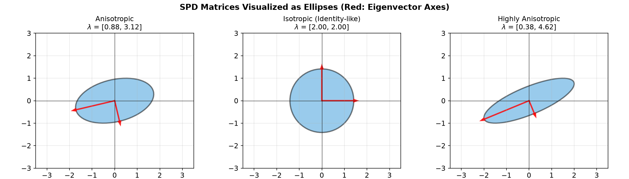
A 2x2 SPD matrix can be visualized as an ellipse. The eigenvectors define the principal axes, and the square roots of eigenvalues define the semi-axis lengths.

import numpy as np
import matplotlib.pyplot as plt
from matplotlib.patches import Ellipse

def create_spd_ellipse(ax, spd_matrix, center=(0, 0), color='blue', alpha=0.5, label=None):
    """Visualize a 2x2 SPD matrix as an ellipse."""
    eigvals, eigvecs = np.linalg.eigh(spd_matrix)
    width = 2 * np.sqrt(eigvals[1])
    height = 2 * np.sqrt(eigvals[0])
    angle = np.degrees(np.arctan2(eigvecs[1, 1], eigvecs[0, 1]))

    ellipse = Ellipse(center, width, height, angle=angle,
                      alpha=alpha, facecolor=color, edgecolor='black', linewidth=2)
    ax.add_patch(ellipse)

    # Draw eigenvalue axes
    for i in range(2):
        vec = eigvecs[:, i] * np.sqrt(eigvals[i])
        ax.arrow(center[0], center[1], vec[0], vec[1],
                 head_width=0.1, color='red', linewidth=2, alpha=0.8)

    if label:
        ax.text(center[0], center[1] - 2.2, label, ha='center', fontsize=10)

# Create SPD matrices with different properties
S1 = np.array([[3.0, 0.5], [0.5, 1.0]])  # Anisotropic
S2 = np.array([[2.0, 0.0], [0.0, 2.0]])  # Isotropic
S3 = np.array([[4.0, 1.5], [1.5, 1.0]])  # Highly anisotropic

fig, axes = plt.subplots(1, 3, figsize=(14, 4))

for ax, S, title in zip(axes, [S1, S2, S3],
    ['Anisotropic', 'Isotropic (Identity-like)', 'Highly Anisotropic']):
    ax.set_xlim(-3.5, 3.5)
    ax.set_ylim(-3, 3)
    ax.set_aspect('equal')
    ax.grid(True, alpha=0.3)
    ax.axhline(y=0, color='k', linewidth=0.5)
    ax.axvline(x=0, color='k', linewidth=0.5)

    eigvals = np.linalg.eigvalsh(S)
    create_spd_ellipse(ax, S, color='#3498db')
    ax.set_title(f'{title}\n$\\lambda$ = [{eigvals[0]:.2f}, {eigvals[1]:.2f}]', fontsize=11)

plt.suptitle('SPD Matrices Visualized as Ellipses (Red: Eigenvector Axes)', fontsize=13, fontweight='bold')
plt.tight_layout()
plt.show()

(Source code)

Why Riemannian Geometry?

SPD matrices do not form a vector space - they form a Riemannian manifold. This has important implications:

• You cannot simply add or average SPD matrices in Euclidean space

• Standard neural network operations may violate the SPD constraint

• Distance metrics like Euclidean distance are not appropriate

The Swelling Effect

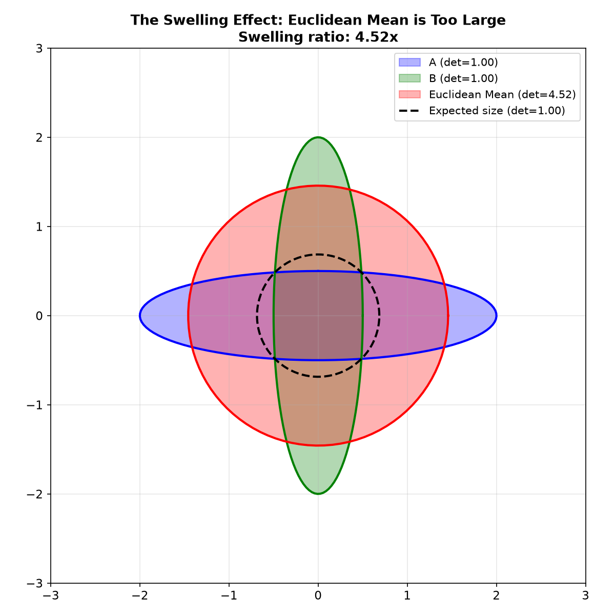
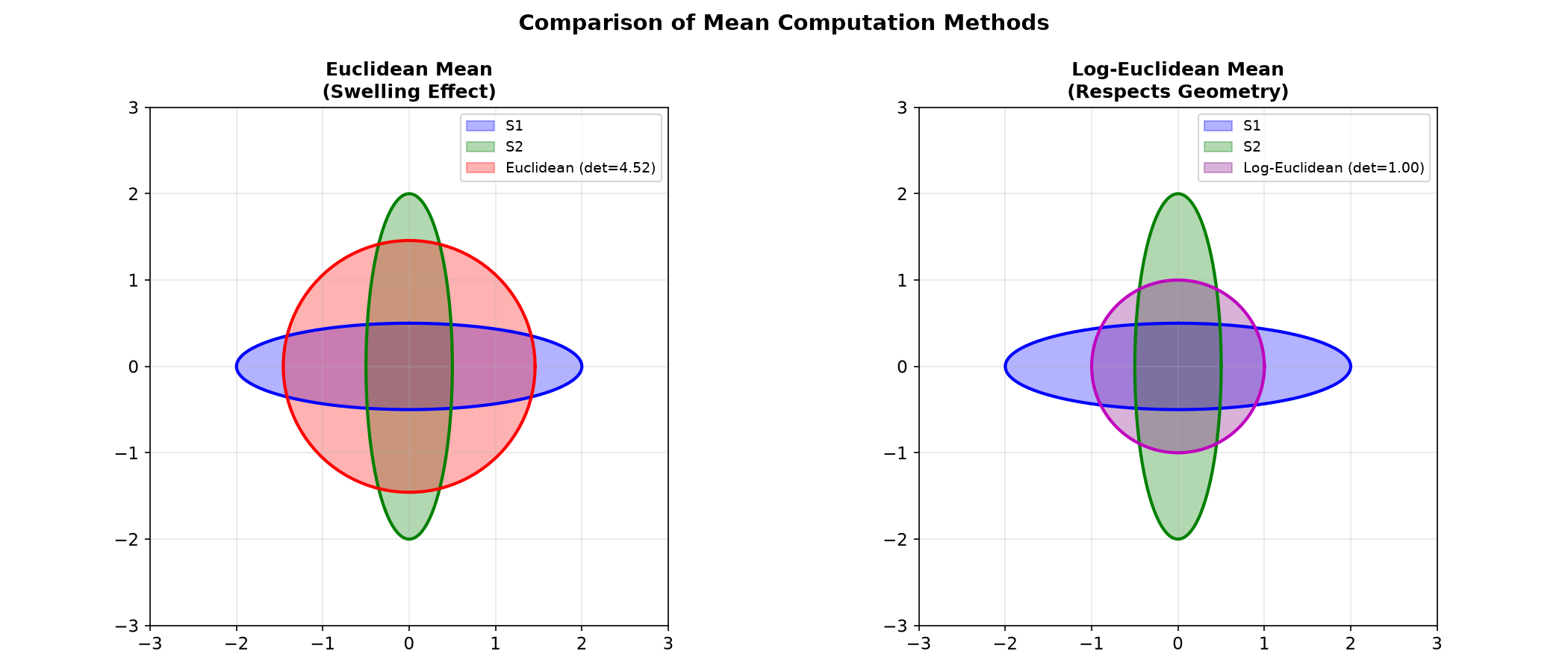
When computing the arithmetic (Euclidean) mean of SPD matrices, the determinant of the mean is often larger than expected. This “swelling effect” violates the intuition that an average should be “in the middle.”

import numpy as np
import matplotlib.pyplot as plt
from matplotlib.patches import Ellipse

def spd_to_ellipse(spd_matrix, n_points=100):
    """Convert 2x2 SPD matrix to ellipse coordinates."""
    eigvals, eigvecs = np.linalg.eigh(spd_matrix)
    theta = np.linspace(0, 2 * np.pi, n_points)
    circle = np.array([np.cos(theta), np.sin(theta)])
    transform = eigvecs @ np.diag(np.sqrt(eigvals))
    ellipse = transform @ circle
    return ellipse[0], ellipse[1]

# Create two very different SPD matrices
A = np.array([[4.0, 0.0], [0.0, 0.25]])  # Large in x, small in y
B = np.array([[0.25, 0.0], [0.0, 4.0]])  # Small in x, large in y

# Euclidean mean
mean_euclidean = (A + B) / 2

# Determinants
det_A = np.linalg.det(A)
det_B = np.linalg.det(B)
det_mean = np.linalg.det(mean_euclidean)
geo_mean_det = np.sqrt(det_A * det_B)

fig, ax = plt.subplots(figsize=(8, 8))

# Plot ellipses
x_A, y_A = spd_to_ellipse(A)
x_B, y_B = spd_to_ellipse(B)
x_mean, y_mean = spd_to_ellipse(mean_euclidean)

ax.fill(x_A, y_A, alpha=0.3, color='blue', label=f'A (det={det_A:.2f})')
ax.plot(x_A, y_A, 'b-', linewidth=2)
ax.fill(x_B, y_B, alpha=0.3, color='green', label=f'B (det={det_B:.2f})')
ax.plot(x_B, y_B, 'g-', linewidth=2)
ax.fill(x_mean, y_mean, alpha=0.3, color='red', label=f'Euclidean Mean (det={det_mean:.2f})')
ax.plot(x_mean, y_mean, 'r-', linewidth=2)

# Reference: ideal size
ideal_scale = np.sqrt(geo_mean_det / det_mean)
ax.plot(x_mean * ideal_scale, y_mean * ideal_scale, 'k--', linewidth=2,
        label=f'Expected size (det={geo_mean_det:.2f})')

ax.set_xlim(-3, 3)
ax.set_ylim(-3, 3)
ax.set_aspect('equal')
ax.grid(True, alpha=0.3)
ax.legend(loc='upper right', fontsize=10)
ax.set_title(f'The Swelling Effect: Euclidean Mean is Too Large\nSwelling ratio: {det_mean/geo_mean_det:.2f}x',
             fontsize=13, fontweight='bold')
plt.tight_layout()
plt.show()

(Source code)

The SPD Manifold Structure

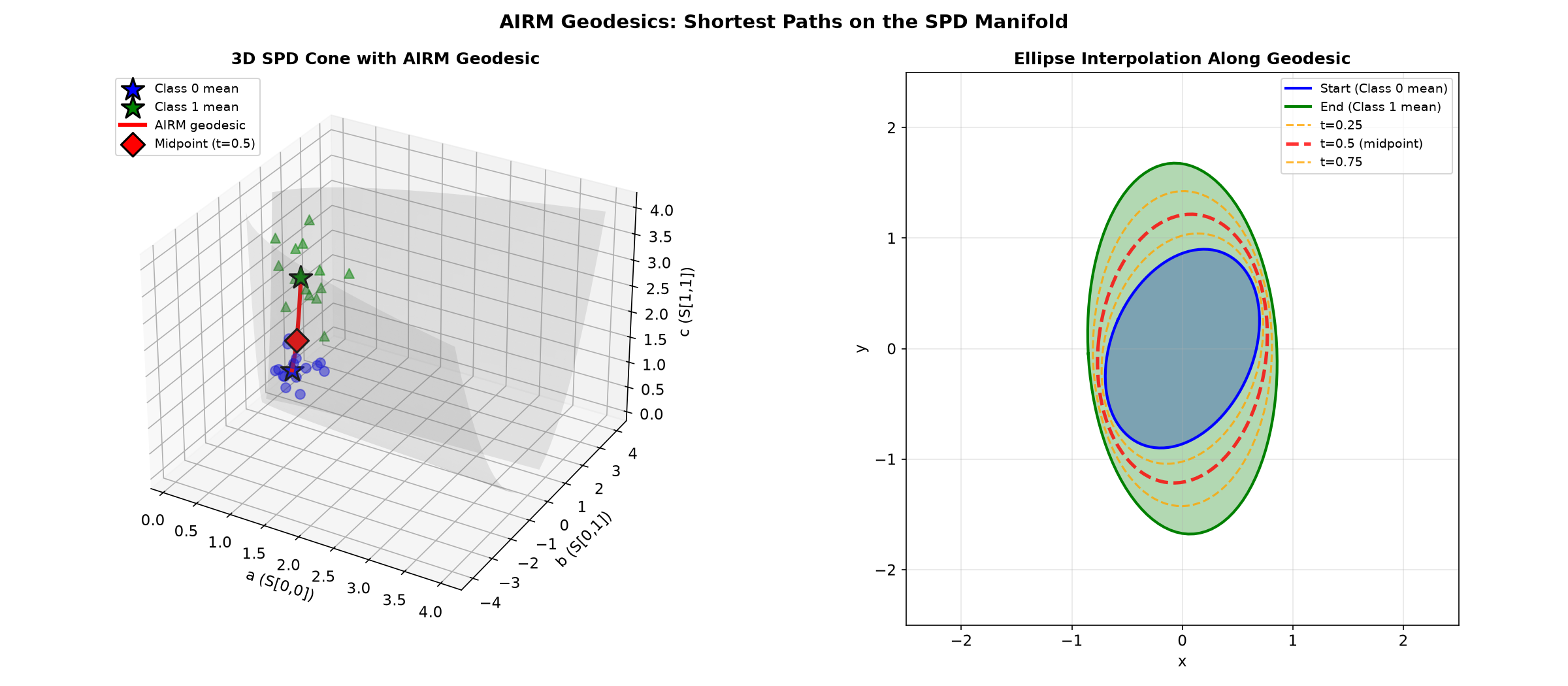
The set of SPD matrices forms an open convex cone. For 2x2 matrices, this can be visualized in 3D where the boundary represents singular matrices.

A 2x2 symmetric matrix \(\begin{bmatrix} a & b \\ b & c \end{bmatrix}\) is SPD when \(a > 0\), \(c > 0\), and \(ac - b^2 > 0\) (positive determinant).

Package Architecture

SPD Learn is organized into three main components:

1. functional - Low-level operations for symmetric and SPD matrices

2. modules - Neural network layers for the SPD manifold

3. models - Pre-built architectures for common tasks

spd_learn/
├── functional/     # Matrix operations (log, exp, eigendecomposition)
├── modules/        # Neural network layers (BiMap, ReEig, LogEig)
└── models/         # Complete architectures (SPDNet, TensorCSPNet, etc.)

Neural Network Modules

SPD Learn provides specialized neural network layers that respect the geometry of the SPD manifold. Each layer is designed to transform SPD matrices while preserving their positive definiteness.

CovLayer: Computing Covariances

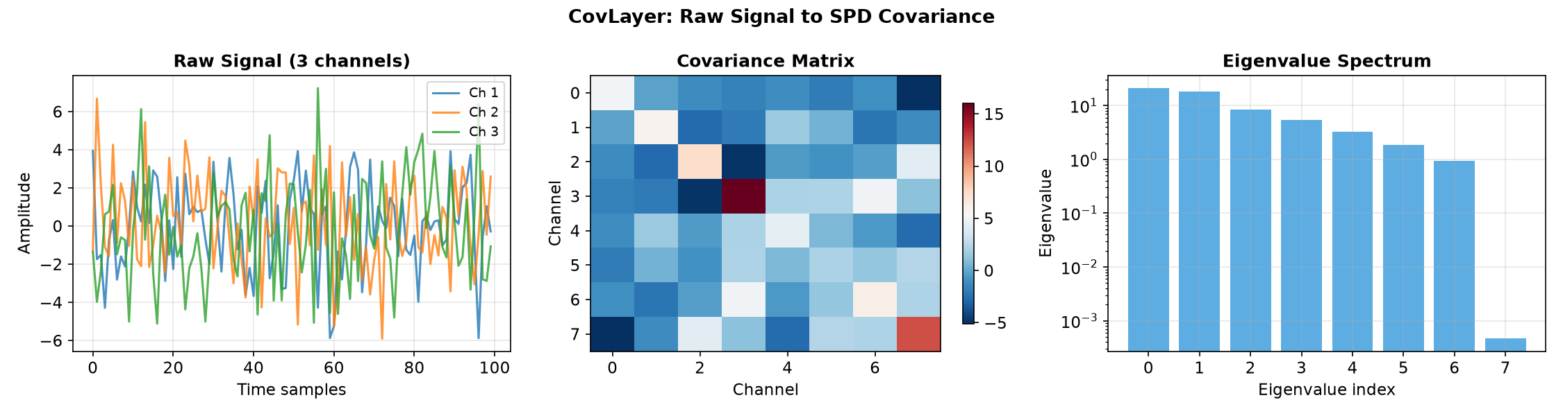
The CovLayer transforms raw multivariate time series into SPD covariance matrices:

\[\Sigma = \mathcal{C}(X)\]

Input: (batch, channels, time)
Output: (batch, channels, channels)

import torch
import numpy as np
import matplotlib.pyplot as plt
from spd_learn.modules import CovLayer

# Generate synthetic multivariate time series
torch.manual_seed(42)
batch_size, n_channels, n_times = 1, 8, 100

# Create correlated signals
raw_signals = torch.randn(batch_size, n_channels, n_times)
mixing_matrix = torch.randn(n_channels, n_channels)
raw_signals = torch.einsum('ij,bjt->bit', mixing_matrix, raw_signals)

# Apply CovLayer
cov_layer = CovLayer()
covariances = cov_layer(raw_signals)

fig, axes = plt.subplots(1, 3, figsize=(15, 4))

# Plot raw signal (first 3 channels)
ax1 = axes[0]
for i in range(3):
    ax1.plot(raw_signals[0, i, :].numpy(), label=f'Ch {i+1}', alpha=0.8)
ax1.set_xlabel('Time samples')
ax1.set_ylabel('Amplitude')
ax1.set_title('Raw Signal (3 channels)', fontweight='bold')
ax1.legend(fontsize=9)
ax1.grid(True, alpha=0.3)

# Plot covariance matrix
ax2 = axes[1]
im = ax2.imshow(covariances[0].numpy(), cmap='RdBu_r', aspect='auto')
ax2.set_title('Covariance Matrix', fontweight='bold')
ax2.set_xlabel('Channel')
ax2.set_ylabel('Channel')
plt.colorbar(im, ax=ax2, shrink=0.8)

# Plot eigenvalue spectrum
ax3 = axes[2]
eigvals = torch.linalg.eigvalsh(covariances[0]).numpy()
ax3.bar(range(n_channels), sorted(eigvals, reverse=True), color='#3498db', alpha=0.8)
ax3.set_xlabel('Eigenvalue index')
ax3.set_ylabel('Eigenvalue')
ax3.set_title('Eigenvalue Spectrum', fontweight='bold')
ax3.set_yscale('log')
ax3.grid(True, alpha=0.3)

plt.suptitle('CovLayer: Raw Signal to SPD Covariance', fontsize=13, fontweight='bold')
plt.tight_layout()
plt.show()

(Source code)

from spd_learn.modules import CovLayer

cov = CovLayer()
# Input: (batch, channels, time) -> Output: (batch, channels, channels)

BiMap Layer: Bilinear Mapping

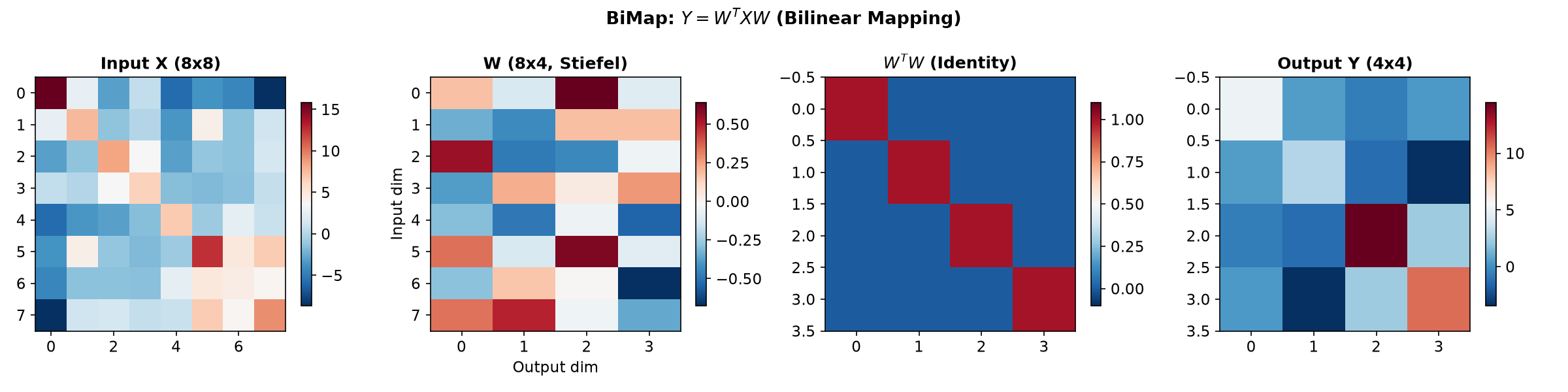
The BiMap layer performs dimensionality reduction while preserving the SPD structure through a bilinear congruence transformation:

\[Y = W^\top X W\]

where \(W \in \reals^{n \times m}\) is a learnable matrix constrained to the Stiefel manifold (\(W^\top W = \I_m\)).

Key properties:

• If X is SPD, then Y is also SPD

• The orthogonality constraint prevents information collapse

• Analogous to a linear layer in standard networks

import torch
import numpy as np
import matplotlib.pyplot as plt
from spd_learn.modules import BiMap

torch.manual_seed(42)

# Create an 8x8 SPD matrix
n_in, n_out = 8, 4
A = torch.randn(n_in, n_in)
X = A @ A.T + 0.1 * torch.eye(n_in)
X = X.unsqueeze(0)  # Add batch dimension

# Apply BiMap
bimap = BiMap(in_features=n_in, out_features=n_out, parametrized=True)
Y = bimap(X)

fig, axes = plt.subplots(1, 4, figsize=(16, 4))

# Input
ax1 = axes[0]
im1 = ax1.imshow(X[0].numpy(), cmap='RdBu_r', aspect='auto')
ax1.set_title(f'Input X ({n_in}x{n_in})', fontweight='bold')
plt.colorbar(im1, ax=ax1, shrink=0.8)

# Weight matrix W
ax2 = axes[1]
W = bimap.weight[0].detach().numpy()
im2 = ax2.imshow(W, cmap='RdBu_r', aspect='auto')
ax2.set_title(f'W ({n_in}x{n_out}, Stiefel)', fontweight='bold')
ax2.set_xlabel('Output dim')
ax2.set_ylabel('Input dim')
plt.colorbar(im2, ax=ax2, shrink=0.8)

# W^T W (should be identity)
ax3 = axes[2]
WtW = (bimap.weight[0].T @ bimap.weight[0]).detach().numpy()
im3 = ax3.imshow(WtW, cmap='RdBu_r', aspect='auto', vmin=-0.1, vmax=1.1)
ax3.set_title(r'$W^T W$ (Identity)', fontweight='bold')
plt.colorbar(im3, ax=ax3, shrink=0.8)

# Output
ax4 = axes[3]
im4 = ax4.imshow(Y[0].detach().numpy(), cmap='RdBu_r', aspect='auto')
ax4.set_title(f'Output Y ({n_out}x{n_out})', fontweight='bold')
plt.colorbar(im4, ax=ax4, shrink=0.8)

plt.suptitle(r'BiMap: $Y = W^T X W$ (Bilinear Mapping)', fontsize=13, fontweight='bold')
plt.tight_layout()
plt.show()

(Source code)

from spd_learn.modules import BiMap

# Reduce from 64x64 to 32x32
bimap = BiMap(in_features=64, out_features=32)

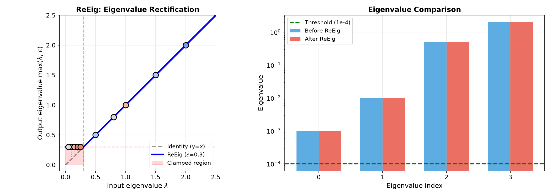
ReEig Layer: Rectified Eigenvalues

The ReEig layer introduces non-linearity by applying a ReLU-like function to eigenvalues:

\[\reeig(X) = U \max(\Lambda, \varepsilon \I) U^\top\]

where \(X = U \Lambda U^\top\) is the eigendecomposition and \(\varepsilon\) is a small threshold.

Geometric interpretation:

• Clamps small eigenvalues to \(\varepsilon\)

• Prevents matrices from becoming singular

• Analogous to ReLU in standard neural networks

import torch
import numpy as np
import matplotlib.pyplot as plt
from matplotlib.patches import Ellipse
from spd_learn.modules import ReEig

# Threshold
epsilon = 0.3

# Create matrices with varying eigenvalues (some below threshold)
eigval_sets = [
    np.array([0.1, 2.0]),   # First below
    np.array([0.5, 1.5]),   # Both above
    np.array([0.05, 0.8]),  # First below
    np.array([1.0, 0.15]),  # Second below
    np.array([0.2, 0.25]),  # Both below
]

fig, axes = plt.subplots(1, 2, figsize=(14, 5))

# Plot ReEig function
ax1 = axes[0]
x = np.linspace(0, 2.5, 200)
y_reeig = np.maximum(x, epsilon)

ax1.plot(x, x, 'k--', alpha=0.4, label='Identity (y=x)', linewidth=2)
ax1.plot(x, y_reeig, 'b-', linewidth=3, label=f'ReEig ($\\epsilon$={epsilon})')
ax1.fill_between([0, epsilon], [epsilon, epsilon], [0, 0],
                 color='red', alpha=0.15, label='Clamped region')
ax1.axhline(y=epsilon, color='red', linestyle='--', alpha=0.5)
ax1.axvline(x=epsilon, color='red', linestyle='--', alpha=0.5)

# Mark example eigenvalues
colors = plt.cm.coolwarm(np.linspace(0.2, 0.8, len(eigval_sets)))
for i, eigvals in enumerate(eigval_sets):
    for ev in eigvals:
        out_ev = max(ev, epsilon)
        ax1.scatter([ev], [out_ev], s=100, c=[colors[i]], edgecolors='black', linewidth=1.5, zorder=5)
        if ev < epsilon:
            ax1.plot([ev, ev], [ev, epsilon], color=colors[i], linestyle=':', linewidth=1.5)

ax1.set_xlim(-0.1, 2.5)
ax1.set_ylim(-0.1, 2.5)
ax1.set_xlabel('Input eigenvalue $\\lambda$', fontsize=12)
ax1.set_ylabel('Output eigenvalue max($\\lambda$, $\\epsilon$)', fontsize=12)
ax1.set_title('ReEig: Eigenvalue Rectification', fontsize=13, fontweight='bold')
ax1.legend(loc='lower right', fontsize=10)
ax1.grid(True, alpha=0.3)
ax1.set_aspect('equal')

# Eigenvalue comparison bar chart
ax2 = axes[1]
demo_eigvals = torch.tensor([2.0, 0.5, 0.01, 0.001])
demo_eigvecs = torch.linalg.qr(torch.randn(4, 4))[0]
demo_spd = demo_eigvecs @ torch.diag(demo_eigvals) @ demo_eigvecs.T
demo_spd = demo_spd.unsqueeze(0)

reeig = ReEig(threshold=1e-4)
demo_rectified = reeig(demo_spd)

eigvals_before = torch.linalg.eigvalsh(demo_spd[0]).numpy()
eigvals_after = torch.linalg.eigvalsh(demo_rectified[0]).numpy()

x_pos = np.arange(4)
width = 0.35
bars1 = ax2.bar(x_pos - width/2, eigvals_before, width, label='Before ReEig', color='#3498db', alpha=0.8)
bars2 = ax2.bar(x_pos + width/2, eigvals_after, width, label='After ReEig', color='#e74c3c', alpha=0.8)
ax2.axhline(y=1e-4, color='green', linestyle='--', linewidth=2, label='Threshold (1e-4)')
ax2.set_xlabel('Eigenvalue index', fontsize=12)
ax2.set_ylabel('Eigenvalue', fontsize=12)
ax2.set_title('Eigenvalue Comparison', fontsize=13, fontweight='bold')
ax2.set_yscale('log')
ax2.set_xticks(x_pos)
ax2.legend(fontsize=10)
ax2.grid(True, alpha=0.3)

plt.tight_layout()
plt.show()

(Source code)

from spd_learn.modules import ReEig

reeig = ReEig(threshold=1e-4)

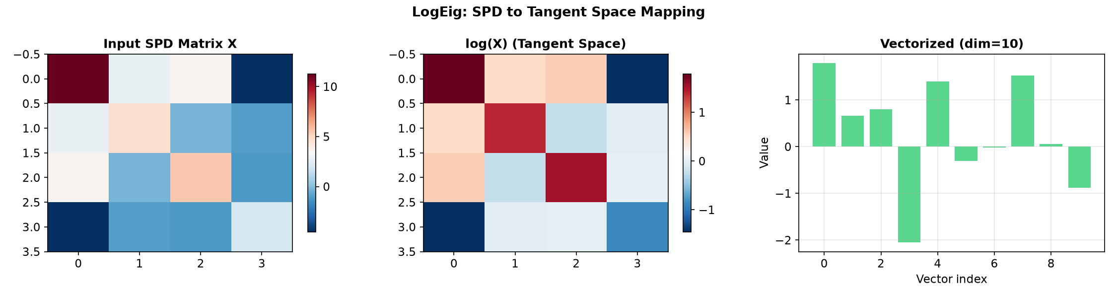
LogEig Layer: Tangent Space Projection

The LogEig layer maps SPD matrices to the tangent space at the identity by applying the matrix logarithm:

\[\log(X) = U \log(\Lambda) U^\top\]

Geometric interpretation:

• Projects from the curved manifold to a flat tangent space

• In the tangent space, standard Euclidean operations apply

• Enables use of standard linear classifiers

import torch
import numpy as np
import matplotlib.pyplot as plt
from spd_learn.modules import LogEig

torch.manual_seed(42)

# Create a 4x4 SPD matrix
n = 4
A = torch.randn(n, n)
X = A @ A.T + 0.1 * torch.eye(n)
X = X.unsqueeze(0)

# Apply LogEig (with and without vectorization)
logeig_full = LogEig(upper=False, flatten=False)
logeig_vec = LogEig(upper=True, flatten=True)

log_matrix = logeig_full(X)
log_vector = logeig_vec(X)

fig, axes = plt.subplots(1, 3, figsize=(15, 4))

# Input SPD matrix
ax1 = axes[0]
im1 = ax1.imshow(X[0].numpy(), cmap='RdBu_r', aspect='auto')
ax1.set_title('Input SPD Matrix X', fontweight='bold')
plt.colorbar(im1, ax=ax1, shrink=0.8)

# Matrix logarithm
ax2 = axes[1]
im2 = ax2.imshow(log_matrix[0].numpy(), cmap='RdBu_r', aspect='auto')
ax2.set_title(r'log(X) (Tangent Space)', fontweight='bold')
plt.colorbar(im2, ax=ax2, shrink=0.8)

# Vectorized output
ax3 = axes[2]
vec = log_vector[0].numpy()
ax3.bar(range(len(vec)), vec, color='#2ecc71', alpha=0.8)
ax3.set_xlabel('Vector index')
ax3.set_ylabel('Value')
ax3.set_title(f'Vectorized (dim={len(vec)})', fontweight='bold')
ax3.grid(True, alpha=0.3)

plt.suptitle('LogEig: SPD to Tangent Space Mapping', fontsize=13, fontweight='bold')
plt.tight_layout()
plt.show()

(Source code)

from spd_learn.modules import LogEig

# Vectorized output for classification
logeig = LogEig(upper=True, flatten=True)

Batch Normalization

SPD Learn provides Riemannian batch normalization layers:

SPDBatchNormMean [Brooks et al., 2019]

Estimates the batch Fréchet mean \(\frechet\) and centers inputs:

\[\tilde{P}_i = \frechet^{-1/2} P_i \frechet^{-1/2}\]

SPDBatchNormMeanVar [Kobler et al., 2022]

Extends SPDBatchNormMean with dispersion normalization.

from spd_learn.modules import SPDBatchNormMeanVar

bn = SPDBatchNormMeanVar(num_features=32, momentum=0.1, affine=True)

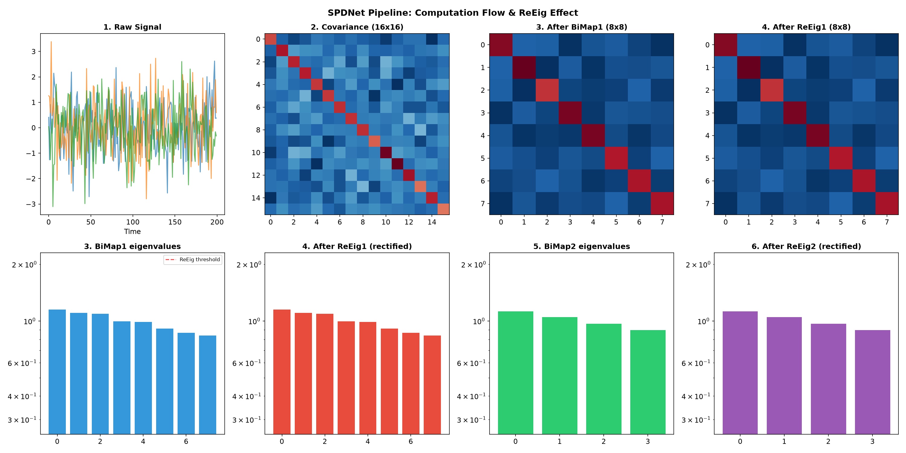
Typical SPDNet Pipeline

Most SPD Learn models follow this general pipeline:

Raw Data --> Covariance --> BiMap --> ReEig --> BiMap --> ReEig --> LogEig --> Linear

import torch
import torch.nn as nn
import numpy as np
import matplotlib.pyplot as plt
from spd_learn.modules import CovLayer, BiMap, ReEig, LogEig, Shrinkage

class SimpleSPDNet(nn.Module):
    """A simple SPD network for demonstration."""

    def __init__(self, n_channels, n_classes):
        super().__init__()
        self.cov = CovLayer()
        self.shrinkage = Shrinkage(n_chans=n_channels, init_shrinkage=0.1)
        self.bimap1 = BiMap(in_features=n_channels, out_features=n_channels // 2)
        self.reeig1 = ReEig()
        self.bimap2 = BiMap(in_features=n_channels // 2, out_features=n_channels // 4)
        self.reeig2 = ReEig()
        self.logeig = LogEig(upper=True)
        tangent_dim = (n_channels // 4) * (n_channels // 4 + 1) // 2
        self.classifier = nn.Linear(tangent_dim, n_classes)

    def forward(self, x, return_intermediates=False):
        intermediates = {}
        x = self.cov(x); intermediates['cov'] = x.clone()
        x = self.shrinkage(x); intermediates['shrinkage'] = x.clone()
        x = self.bimap1(x); intermediates['bimap1'] = x.clone()
        x = self.reeig1(x); intermediates['reeig1'] = x.clone()
        x = self.bimap2(x); intermediates['bimap2'] = x.clone()
        x = self.reeig2(x); intermediates['reeig2'] = x.clone()
        x = self.logeig(x); intermediates['logeig'] = x.clone()
        x = self.classifier(x); intermediates['output'] = x.clone()
        if return_intermediates:
            return x, intermediates
        return x

# Create and run the network
torch.manual_seed(42)
n_channels, n_classes = 16, 4
model = SimpleSPDNet(n_channels=n_channels, n_classes=n_classes)

raw_input = torch.randn(1, n_channels, 200)
output, intermediates = model(raw_input, return_intermediates=True)

# Visualize the pipeline in computation order
fig, axes = plt.subplots(2, 4, figsize=(20, 10))

# Row 1: Matrix representations (computation order)
ax1 = axes[0, 0]
ax1.plot(raw_input[0, :3, :].T.numpy(), alpha=0.7)
ax1.set_title('1. Raw Signal', fontweight='bold')
ax1.set_xlabel('Time')

ax2 = axes[0, 1]
im2 = ax2.imshow(intermediates['cov'][0].detach().numpy(), cmap='RdBu_r', aspect='auto')
ax2.set_title('2. Covariance (16x16)', fontweight='bold')

ax3 = axes[0, 2]
im3 = ax3.imshow(intermediates['bimap1'][0].detach().numpy(), cmap='RdBu_r', aspect='auto')
ax3.set_title('3. After BiMap1 (8x8)', fontweight='bold')

ax4 = axes[0, 3]
im4 = ax4.imshow(intermediates['reeig1'][0].detach().numpy(), cmap='RdBu_r', aspect='auto')
ax4.set_title('4. After ReEig1 (8x8)', fontweight='bold')

# Row 2: Show ReEig effect with before/after eigenvalue comparison
eigvals_bimap1 = torch.linalg.eigvalsh(intermediates['bimap1'][0]).detach().numpy()
eigvals_reeig1 = torch.linalg.eigvalsh(intermediates['reeig1'][0]).detach().numpy()
eigvals_bimap2 = torch.linalg.eigvalsh(intermediates['bimap2'][0]).detach().numpy()
eigvals_reeig2 = torch.linalg.eigvalsh(intermediates['reeig2'][0]).detach().numpy()

# Compute shared y-limits across all eigenvalue plots
all_eigvals = np.concatenate([eigvals_bimap1, eigvals_reeig1, eigvals_bimap2, eigvals_reeig2])
y_min, y_max = max(all_eigvals[all_eigvals > 0].min() * 0.3, 1e-6), all_eigvals.max() * 2

ax5 = axes[1, 0]
ax5.bar(range(len(eigvals_bimap1)), sorted(eigvals_bimap1, reverse=True), color='#3498db')
ax5.set_title('3. BiMap1 eigenvalues', fontweight='bold')
ax5.set_yscale('log')
ax5.set_ylim(y_min, y_max)
ax5.axhline(y=1e-4, color='red', linestyle='--', alpha=0.7, label='ReEig threshold')
ax5.legend(loc='upper right', fontsize=8)

ax6 = axes[1, 1]
ax6.bar(range(len(eigvals_reeig1)), sorted(eigvals_reeig1, reverse=True), color='#e74c3c')
ax6.set_title('4. After ReEig1 (rectified)', fontweight='bold')
ax6.set_yscale('log')
ax6.set_ylim(y_min, y_max)
ax6.axhline(y=1e-4, color='red', linestyle='--', alpha=0.7)

ax7 = axes[1, 2]
ax7.bar(range(len(eigvals_bimap2)), sorted(eigvals_bimap2, reverse=True), color='#2ecc71')
ax7.set_title('5. BiMap2 eigenvalues', fontweight='bold')
ax7.set_yscale('log')
ax7.set_ylim(y_min, y_max)
ax7.axhline(y=1e-4, color='red', linestyle='--', alpha=0.7)

ax8 = axes[1, 3]
ax8.bar(range(len(eigvals_reeig2)), sorted(eigvals_reeig2, reverse=True), color='#9b59b6')
ax8.set_title('6. After ReEig2 (rectified)', fontweight='bold')
ax8.set_yscale('log')
ax8.set_ylim(y_min, y_max)
ax8.axhline(y=1e-4, color='red', linestyle='--', alpha=0.7)

plt.suptitle('SPDNet Pipeline: Computation Flow & ReEig Effect', fontsize=14, fontweight='bold')
plt.tight_layout()
plt.show()

(Source code)

import torch
from spd_learn.models import SPDNet

model = SPDNet(
    n_chans=64,  # Number of channels
    n_outputs=4,  # Number of classes
    input_type="raw",
    subspacedim=32,
)

x = torch.randn(16, 64, 1000)  # (batch, channels, time)
output = model(x)  # (batch, n_outputs)

Log-Euclidean Operations

SPD Learn provides operations based on the Log-Euclidean metric, which respects the manifold structure while being computationally efficient.

Matrix Logarithm and Exponential

\[\log(S) = U \log(\Lambda) U^\top, \quad \exp(X) = U \exp(\Lambda) U^\top\]

Log-Euclidean Distance

\[\dlem{A}{B} = \frob{\log(A) - \log(B)}\]

Log-Euclidean Mean

\[\bar{S}_{LE} = \exp\left(\frac{1}{n}\sum_{i=1}^n \log(S_i)\right)\]

import torch
import numpy as np
import matplotlib.pyplot as plt
from spd_learn.functional import matrix_log, matrix_exp, log_euclidean_mean

def spd_to_ellipse(spd_matrix, n_points=100):
    eigvals, eigvecs = np.linalg.eigh(spd_matrix)
    theta = np.linspace(0, 2 * np.pi, n_points)
    circle = np.array([np.cos(theta), np.sin(theta)])
    transform = eigvecs @ np.diag(np.sqrt(eigvals))
    ellipse = transform @ circle
    return ellipse[0], ellipse[1]

# Create two SPD matrices
S1 = torch.tensor([[4.0, 0.0], [0.0, 0.25]], dtype=torch.float64)
S2 = torch.tensor([[0.25, 0.0], [0.0, 4.0]], dtype=torch.float64)

# Euclidean mean
mean_euclidean = (S1 + S2) / 2

# Log-Euclidean mean
S_stack = torch.stack([S1, S2], dim=0)
weights = torch.tensor([[0.5, 0.5]], dtype=torch.float64)
mean_log_euclidean = log_euclidean_mean(weights, S_stack).squeeze(0)

fig, axes = plt.subplots(1, 2, figsize=(14, 6))

# Convert to numpy
S1_np, S2_np = S1.numpy(), S2.numpy()
mean_euc_np = mean_euclidean.numpy()
mean_le_np = mean_log_euclidean.numpy()

# Euclidean mean
ax1 = axes[0]
for S, color, label in [(S1_np, 'blue', 'S1'), (S2_np, 'green', 'S2')]:
    x, y = spd_to_ellipse(S)
    ax1.fill(x, y, alpha=0.3, color=color, label=label)
    ax1.plot(x, y, color=color, linewidth=2)
x, y = spd_to_ellipse(mean_euc_np)
ax1.fill(x, y, alpha=0.3, color='red', label=f'Euclidean (det={np.linalg.det(mean_euc_np):.2f})')
ax1.plot(x, y, 'r-', linewidth=2)
ax1.set_xlim(-3, 3); ax1.set_ylim(-3, 3)
ax1.set_aspect('equal'); ax1.grid(True, alpha=0.3)
ax1.legend(loc='upper right', fontsize=9)
ax1.set_title('Euclidean Mean\n(Swelling Effect)', fontsize=12, fontweight='bold')

# Log-Euclidean mean
ax2 = axes[1]
for S, color, label in [(S1_np, 'blue', 'S1'), (S2_np, 'green', 'S2')]:
    x, y = spd_to_ellipse(S)
    ax2.fill(x, y, alpha=0.3, color=color, label=label)
    ax2.plot(x, y, color=color, linewidth=2)
x, y = spd_to_ellipse(mean_le_np)
ax2.fill(x, y, alpha=0.3, color='purple', label=f'Log-Euclidean (det={np.linalg.det(mean_le_np):.2f})')
ax2.plot(x, y, 'm-', linewidth=2)
ax2.set_xlim(-3, 3); ax2.set_ylim(-3, 3)
ax2.set_aspect('equal'); ax2.grid(True, alpha=0.3)
ax2.legend(loc='upper right', fontsize=9)
ax2.set_title('Log-Euclidean Mean\n(Respects Geometry)', fontsize=12, fontweight='bold')

plt.suptitle('Comparison of Mean Computation Methods', fontsize=14, fontweight='bold')
plt.tight_layout()
plt.show()

(Source code)

AIRM Geodesics on the SPD Manifold

The Affine-Invariant Riemannian Metric (AIRM) provides geodesics that stay within the SPD cone. The geodesic between SPD matrices \(A\) and \(B\) is given by:

\[\gamma(t) = A^{1/2} (A^{-1/2} B A^{-1/2})^t A^{1/2}\]

This ensures all intermediate points remain positive definite.

import torch
import numpy as np
import matplotlib.pyplot as plt
from mpl_toolkits.mplot3d import Axes3D
from pyriemann.datasets import make_gaussian_blobs
from spd_learn.functional import airm_geodesic, airm_distance, log_euclidean_mean, matrix_log, matrix_exp

# Helper: map 2x2 SPD [[a,b],[b,c]] to 3D coords (a, b, c)
def spd_to_3d_coords(S):
    if isinstance(S, torch.Tensor):
        S = S.numpy()
    return S[0, 0], S[0, 1], S[1, 1]

# Helper: convert SPD to ellipse for 2D visualization
def spd_to_ellipse(spd_matrix, n_points=100):
    if isinstance(spd_matrix, torch.Tensor):
        spd_matrix = spd_matrix.numpy()
    eigvals, eigvecs = np.linalg.eigh(spd_matrix)
    theta = np.linspace(0, 2 * np.pi, n_points)
    circle = np.array([np.cos(theta), np.sin(theta)])
    transform = eigvecs @ np.diag(np.sqrt(eigvals))
    ellipse = transform @ circle
    return ellipse[0], ellipse[1]

# Generate synthetic 2x2 SPD matrices using pyriemann
np.random.seed(42)
X_spd, y = make_gaussian_blobs(
    n_matrices=15, n_dim=2, class_sep=1.5, class_disp=0.5,
    random_state=42, n_jobs=1
)
X_tensor = torch.tensor(X_spd, dtype=torch.float64)

# Separate by class
class0_mask = y == 0
class1_mask = y == 1
X_class0 = X_tensor[class0_mask]
X_class1 = X_tensor[class1_mask]

# Compute class means using Log-Euclidean mean
# For unweighted mean: average in log-domain, then exp back
mean0 = matrix_exp.apply(matrix_log.apply(X_class0).mean(dim=0))
mean1 = matrix_exp.apply(matrix_log.apply(X_class1).mean(dim=0))

# Use class means as start/end of geodesic
A, B = mean0, mean1

# Compute geodesic points and verify eigenvalues stay positive
t_values = [0.0, 0.25, 0.5, 0.75, 1.0]
geodesic_points = []
print("Eigenvalues along AIRM geodesic (all positive = stays in SPD cone):")
for t in t_values:
    G_t = airm_geodesic(A, B, torch.tensor(t))
    geodesic_points.append(G_t)
    eigvals = torch.linalg.eigvalsh(G_t).numpy()
    print(f"  t={t:.2f}: eigenvalues = [{eigvals[0]:.4f}, {eigvals[1]:.4f}]")

# Compute AIRM distance
dist = airm_distance(A.unsqueeze(0), B.unsqueeze(0)).item()
print(f"\nAIRM distance between class means: {dist:.4f}")

# Create figure with 3D cone (left) and 2D ellipses (right)
fig = plt.figure(figsize=(16, 7))

# === Left panel: 3D SPD cone visualization ===
ax1 = fig.add_subplot(121, projection='3d')

# Draw cone boundary surface: det = ac - b^2 = 0
a_range = np.linspace(0.1, 4, 30)
c_range = np.linspace(0.1, 4, 30)
A_grid, C_grid = np.meshgrid(a_range, c_range)
B_pos = np.sqrt(A_grid * C_grid)  # b = sqrt(ac) for det=0
B_neg = -np.sqrt(A_grid * C_grid)

ax1.plot_surface(A_grid, B_pos, C_grid, alpha=0.15, color='gray')
ax1.plot_surface(A_grid, B_neg, C_grid, alpha=0.15, color='gray')

# Plot data points by class
for S in X_class0:
    a, b, c = spd_to_3d_coords(S)
    ax1.scatter(a, b, c, c='blue', marker='o', s=50, alpha=0.7)
for S in X_class1:
    a, b, c = spd_to_3d_coords(S)
    ax1.scatter(a, b, c, c='green', marker='^', s=50, alpha=0.7)

# Plot class means as stars
a0, b0, c0 = spd_to_3d_coords(mean0)
a1, b1, c1 = spd_to_3d_coords(mean1)
ax1.scatter(a0, b0, c0, c='blue', marker='*', s=300, edgecolor='black', linewidth=1.5, label='Class 0 mean', zorder=5)
ax1.scatter(a1, b1, c1, c='green', marker='*', s=300, edgecolor='black', linewidth=1.5, label='Class 1 mean', zorder=5)

# Plot geodesic curve with many points for smoothness
t_fine = np.linspace(0, 1, 50)
geo_coords = []
for t in t_fine:
    G_t = airm_geodesic(A, B, torch.tensor(t))
    geo_coords.append(spd_to_3d_coords(G_t))
geo_coords = np.array(geo_coords)
ax1.plot(geo_coords[:, 0], geo_coords[:, 1], geo_coords[:, 2],
         'r-', linewidth=3, label='AIRM geodesic', zorder=10)

# Mark midpoint
mid = airm_geodesic(A, B, torch.tensor(0.5))
am, bm, cm = spd_to_3d_coords(mid)
ax1.scatter(am, bm, cm, c='red', marker='D', s=150, edgecolor='black', linewidth=1.5, label='Midpoint (t=0.5)', zorder=15)

ax1.set_xlabel('a (S[0,0])', fontsize=11)
ax1.set_ylabel('b (S[0,1])', fontsize=11)
ax1.set_zlabel('c (S[1,1])', fontsize=11)
ax1.set_title('3D SPD Cone with AIRM Geodesic', fontsize=12, fontweight='bold')
ax1.legend(loc='upper left', fontsize=9)

# === Right panel: 2D ellipse interpolation ===
ax2 = fig.add_subplot(122)

# Plot start and end ellipses (filled)
x, y = spd_to_ellipse(A)
ax2.fill(x, y, alpha=0.3, color='blue')
ax2.plot(x, y, 'b-', linewidth=2, label='Start (Class 0 mean)')

x, y = spd_to_ellipse(B)
ax2.fill(x, y, alpha=0.3, color='green')
ax2.plot(x, y, 'g-', linewidth=2, label='End (Class 1 mean)')

# Plot intermediate geodesic ellipses
for t in [0.25, 0.5, 0.75]:
    G_t = airm_geodesic(A, B, torch.tensor(t))
    x, y = spd_to_ellipse(G_t)
    alpha_val = 0.5 if t == 0.5 else 0.25
    lw = 2.5 if t == 0.5 else 1.5
    color = 'red' if t == 0.5 else 'orange'
    label = f't={t} (midpoint)' if t == 0.5 else f't={t}'
    ax2.plot(x, y, color=color, linewidth=lw, linestyle='--', alpha=0.8, label=label)

ax2.set_xlim(-2.5, 2.5)
ax2.set_ylim(-2.5, 2.5)
ax2.set_aspect('equal')
ax2.grid(True, alpha=0.3)
ax2.legend(loc='upper right', fontsize=9)
ax2.set_title('Ellipse Interpolation Along Geodesic', fontsize=12, fontweight='bold')
ax2.set_xlabel('x', fontsize=11)
ax2.set_ylabel('y', fontsize=11)

plt.suptitle('AIRM Geodesics: Shortest Paths on the SPD Manifold', fontsize=14, fontweight='bold')
plt.tight_layout()
plt.show()

(Source code)

Available Models

SPD Learn provides several pre-built architectures:

Model	Description
SPDNet	Deep learning architecture for processing SPD matrices
TensorCSPNet	Geometric deep learning framework capturing temporospatiofrequency patterns on SPD manifolds
TSMNet	Combines convolutional feature extractor, covariance pooling, SPDNet, and Tangent Space Mapping
MAtt	Manifold attention network integrating Riemannian geometry with attention mechanisms
Green	Gabor Riemann EEGNet for processing EEG epochs
EEGSPDNet	EEG signal classification with channel-specific convolution and covariance pooling
PhaseSPDNet	Applies Phase-Space Embedding followed by SPDNet for classification

Integration with Ecosystems

SPD Learn is designed as a natural extension of the established Python ecosystem for brain signal analysis. The library builds upon and integrates with tools developed by the same research community over the past decade:

• pyRiemann (2015): Classical Riemannian methods for BCI, co-developed by members of this research community, laid the foundation for geometric approaches to EEG classification.

• MOABB (2018): The benchmarking standard for BCI algorithms, enabling reproducible comparisons across methods and datasets.

• Braindecode (2017): Deep learning for EEG, providing the EEGClassifier wrapper that SPD Learn models use for scikit-learn compatibility.

• Nilearn: Machine learning for neuroimaging, particularly fMRI connectivity analysis.

This integration reflects the long-term collaborative research effort at institutions including INRIA, CNRS, CEA, Université Paris-Saclay, Université Savoie Mont-Blanc, and RIKEN, bridging classical Riemannian geometry with modern deep learning for neural decoding.

MOABB (EEG)

SPD Learn integrates with MOABB for EEG benchmarking:

from moabb.datasets import BNCI2014_001
from moabb.paradigms import MotorImagery
from braindecode import EEGClassifier
from spd_learn.models import TensorCSPNet

dataset = BNCI2014_001()
paradigm = MotorImagery()
model = SPDNet(
    n_chans=22,  # Number of channels
    n_outputs=4,  # Number of classes
    input_type="raw",
    subspacedim=32,
)

clf = EEGClassifier(
    module=model,
    criterion=torch.nn.CrossEntropyLoss,
    optimizer=torch.optim.Adam,
)

Nilearn (fMRI)

SPD Learn works with Nilearn for fMRI analysis:

from nilearn import datasets
from nilearn.connectome import ConnectivityMeasure
from spd_learn.models import SPDNet

connectivity = ConnectivityMeasure(kind="covariance")
X = connectivity.fit_transform(time_series)

model = SPDNet(n_chans=200, n_outputs=2, input_type="cov")

Next Steps

• Tutorials: See the tutorials for hands-on examples

• Visualizations: Explore layer animations to build intuition

• API Reference: Check the API Reference for detailed documentation

References

[1]

Zhiwu Huang and Luc Van Gool. A riemannian network for spd matrix learning. In Proceedings of the AAAI Conference on Artificial Intelligence, volume 31, 2036–2042. 2017. URL: https://ojs.aaai.org/index.php/AAAI/article/view/10866.

[2]

Ce Ju and Cuntai Guan. Tensor-cspnet: a novel geometric deep learning framework for motor imagery classification. IEEE Transactions on Neural Networks and Learning Systems, 34(12):10955–10969, 2023. doi:10.1109/TNNLS.2022.3172108.

[3] (1,2)

Reinmar J Kobler, Jun-ichiro Hirayama, Qibin Zhao, and Motoaki Kawanabe. Spd domain-specific batch normalization to crack interpretable unsupervised domain adaptation in eeg. In Advances in Neural Information Processing Systems, volume 35, 6219–6235. 2022. URL: https://proceedings.neurips.cc/paper_files/paper/2022/hash/28ef7ee7cd3e03093acc39e1272411b7-Abstract-Conference.html.

[4]

Igor Carrara*, Bruno Aristimunha*, Marie-Constance Corsi, Raphael Y. de Camargo, Sylvain Chevallier, and Théodore Papadopoulo. Geometric neural network based on phase space for bci-eeg decoding. Journal of Neural Engineering, 21(6):016049, 2024. doi:10.1088/1741-2552/ad88a2.

[5]

Antoine Collas, Ce Ju, Nicolas Salvy, and Bertrand Thirion. Riemannian flow matching for brain connectivity matrices via pullback geometry. In The Thirty-ninth Annual Conference on Neural Information Processing Systems. 2025. URL: https://openreview.net/forum?id=NY3LzmUXl7.

[6] (1,2)

Daniel Brooks, Olivier Schwander, Frédéric Barbaresco, Jean-Yves Schneider, and Matthieu Cord. Riemannian batch normalization for spd neural networks. In Advances in Neural Information Processing Systems, volume 32. 2019. URL: https://proceedings.neurips.cc/paper/2019/hash/6e69ebbfad976d4637bb4b39de261bf7-Abstract.html.