CovLayer Animation

This animation visualizes how the CovLayer transforms multivariate time series data into SPD covariance matrices.

\[\Sigma = \frac{1}{T-1} (X - \bar{X})(X - \bar{X})^T\]

where \(X \in \mathbb{R}^{C \times T}\) is the input signal.

# sphinx_gallery_thumbnail_number = 1

Understanding CovLayer

CovLayer is the “entry point” to SPD networks. It converts time series (like EEG signals) into covariance matrices, which capture:

• Variances: Signal power in each channel

• Covariances: Relationships between channels

The resulting matrix is symmetric positive definite (SPD), which can then be processed by SPDNet layers.

import sys

from pathlib import Path

import matplotlib.animation as animation
import matplotlib.pyplot as plt
import numpy as np


# Handle both direct execution and import
try:
    _current_dir = Path(__file__).parent
except NameError:
    _current_dir = Path.cwd() / "examples" / "visualizations"

if str(_current_dir) not in sys.path:
    sys.path.insert(0, str(_current_dir))

from spd_visualization_utils import COLORS, create_ellipse_patch, setup_spd_plot

Setup and Data Generation

np.random.seed(42)

n_channels = 2  # Using 2 channels for ellipsoid visualization
n_times = 200
fs = 100  # Sampling frequency

t = np.linspace(0, n_times / fs, n_times)

# Create correlated signals (simulating EEG)
# Channel 1: 10 Hz oscillation + noise
freq1 = 10
signal1 = np.sin(2 * np.pi * freq1 * t) + 0.3 * np.random.randn(n_times)

# Channel 2: Correlated with channel 1 + different frequency component
freq2 = 12
correlation = 0.7
signal2 = (
    correlation * signal1
    + np.sqrt(1 - correlation**2) * np.sin(2 * np.pi * freq2 * t)
    + 0.3 * np.random.randn(n_times)
)

# Stack into signal matrix
X = np.stack([signal1, signal2])  # Shape: (2, n_times)

# Compute covariance matrix
X_centered = X - X.mean(axis=1, keepdims=True)
cov_matrix = (X_centered @ X_centered.T) / (n_times - 1)

print(f"Signal shape: {X.shape}")
print(f"Covariance matrix:\n{cov_matrix}")
print(f"Eigenvalues: {np.linalg.eigvalsh(cov_matrix)}")

Signal shape: (2, 200)
Covariance matrix:
[[0.55416524 0.39290976]
 [0.39290976 0.6460468 ]]
Eigenvalues: [0.20451957 0.99569247]

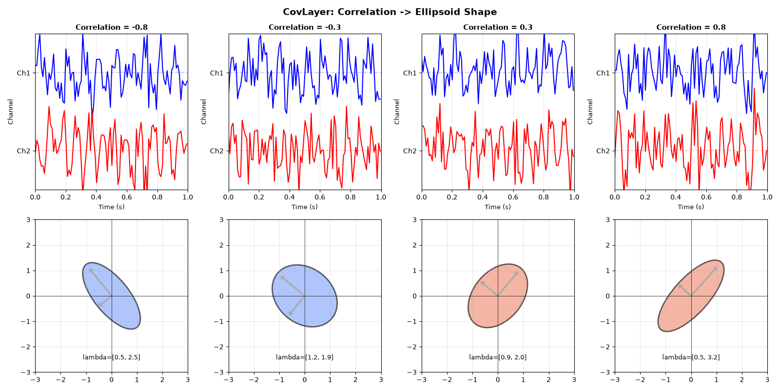
Static Visualization: Multiple Trials

First, let’s see how different correlations produce different ellipsoids.

fig_static, axes_static = plt.subplots(2, 4, figsize=(16, 8))

# Generate multiple "trials" with different correlations
correlations = [-0.8, -0.3, 0.3, 0.8]
np.random.seed(42)

for i, corr in enumerate(correlations):
    # Generate correlated signals
    s1 = np.random.randn(n_times) + np.sin(2 * np.pi * 10 * t)
    s2 = (
        corr * s1
        + np.sqrt(1 - corr**2) * np.random.randn(n_times)
        + np.sin(2 * np.pi * 12 * t)
    )
    trial_X = np.stack([s1, s2])

    # Compute covariance
    trial_X_centered = trial_X - trial_X.mean(axis=1, keepdims=True)
    trial_cov = (trial_X_centered @ trial_X_centered.T) / (n_times - 1)

    # Plot signal (EEG-style with vertical offset)
    ax_top = axes_static[0, i]
    channel_offset = 2.5  # Vertical separation between channels
    ax_top.plot(
        t[:100], trial_X[0, :100] + channel_offset, "b-", linewidth=1.5, label="Ch1"
    )
    ax_top.plot(
        t[:100], trial_X[1, :100] - channel_offset, "r-", linewidth=1.5, label="Ch2"
    )
    ax_top.axhline(y=channel_offset, color="b", linestyle="--", alpha=0.2)
    ax_top.axhline(y=-channel_offset, color="r", linestyle="--", alpha=0.2)
    ax_top.set_title(f"Correlation = {corr:.1f}", fontsize=11, fontweight="bold")
    ax_top.set_xlabel("Time (s)", fontsize=9)
    ax_top.set_ylabel("Channel", fontsize=9)
    ax_top.set_yticks([channel_offset, -channel_offset])
    ax_top.set_yticklabels(["Ch1", "Ch2"])
    ax_top.set_xlim(0, 1)
    ax_top.set_ylim(-5, 5)
    ax_top.grid(True, alpha=0.3, axis="x")

    # Plot ellipsoid
    ax_bot = axes_static[1, i]
    setup_spd_plot(ax_bot, xlim=(-3, 3), ylim=(-3, 3), title="")

    # Determine color based on correlation
    if corr < 0:
        color = plt.cm.coolwarm(0.2)
    elif corr > 0:
        color = plt.cm.coolwarm(0.8)
    else:
        color = plt.cm.coolwarm(0.5)

    ellipse = create_ellipse_patch(
        trial_cov,
        (0, 0),
        alpha=0.6,
        color=color,
        edgecolor="black",
        linewidth=2,
    )
    ax_bot.add_patch(ellipse)

    # Eigenvectors
    eigvals, eigvecs = np.linalg.eigh(trial_cov)
    for j in range(2):
        vec = eigvecs[:, j] * np.sqrt(eigvals[j]) * 0.8
        ax_bot.arrow(
            0,
            0,
            vec[0],
            vec[1],
            head_width=0.12,
            head_length=0.08,
            fc="darkgray",
            ec="darkgray",
            linewidth=2,
        )

    ax_bot.text(
        0, -2.5, f"lambda=[{eigvals[0]:.1f}, {eigvals[1]:.1f}]", ha="center", fontsize=9
    )

fig_static.suptitle(
    "CovLayer: Correlation -> Ellipsoid Shape", fontsize=14, fontweight="bold"
)
plt.tight_layout()

Regularization for SPD

When the number of time points is small, we need regularization to ensure the covariance matrix is positive definite.

fig_reg, axes_reg = plt.subplots(1, 3, figsize=(14, 4))

# Show effect of regularization
epsilon_values = [0, 0.1, 0.5]

# Create a rank-deficient covariance (e.g., n_times < n_channels scenario)
np.random.seed(42)
X_short = np.random.randn(2, 3)  # Only 3 time points for 2 channels
X_short_centered = X_short - X_short.mean(axis=1, keepdims=True)
cov_rank_def = (X_short_centered @ X_short_centered.T) / 2  # Rank-deficient

print("\nRank-deficient covariance (n_times=3, n_channels=2):")
print(f"Eigenvalues: {np.linalg.eigvalsh(cov_rank_def)}")

for i, eps in enumerate(epsilon_values):
    ax = axes_reg[i]

    # Regularized covariance
    cov_reg = cov_rank_def + eps * np.eye(2)
    eigvals = np.linalg.eigvalsh(cov_reg)

    setup_spd_plot(
        ax,
        xlim=(-3, 3),
        ylim=(-3, 3),
        title=f"epsilon = {eps} (lambda = [{eigvals[0]:.2f}, {eigvals[1]:.2f}])",
    )

    if np.all(eigvals > 1e-10):
        ellipse = create_ellipse_patch(
            cov_reg,
            (0, 0),
            alpha=0.6,
            color="green" if eps > 0 else "red",
            edgecolor="black",
            linewidth=2,
        )
        ax.add_patch(ellipse)
        status = "SPD (valid)" if eps > 0 else "PSD (boundary)"
    else:
        status = "Singular (invalid)"

    ax.text(
        0,
        -2.5,
        status,
        ha="center",
        fontsize=11,
        fontweight="bold",
        color="green" if eps > 0 else "red",
    )

fig_reg.suptitle(
    "Regularization: Adding epsilon*I for Numerical Stability",
    fontsize=14,
    fontweight="bold",
)
plt.tight_layout()

Rank-deficient covariance (n_times=3, n_channels=2):
Eigenvalues: [0.15107105 1.05210243]

Mathematical Explanation

The CovLayer performs:

\[\Sigma = \frac{1}{T-1} (X - \bar{X})(X - \bar{X})^T\]

Properties of the output:

• Symmetric: \(\Sigma = \Sigma^T\)

• Positive semi-definite: All eigenvalues \(\geq 0\)

• With regularization: Positive definite (all eigenvalues > 0)

The covariance matrix captures:

• Diagonal elements (variances): Signal power per channel

• Off-diagonal elements (covariances): Linear relationships

Ellipsoid interpretation:

• Shape: Elongated = high variance along eigenvector direction

• Orientation: Principal axes = eigenvectors

• Size: Overall variance (trace)

Animation

The animation shows CovLayer computing covariances in real-time using a sliding window over the time series.

# Create animation figure
fig_anim = plt.figure(figsize=(10, 4), dpi=60)

# Three subplots: time series, covariance matrix, ellipsoid
ax_signal = fig_anim.add_subplot(1, 3, 1)
ax_cov = fig_anim.add_subplot(1, 3, 2)
ax_ellipse = fig_anim.add_subplot(1, 3, 3)

# Animation parameters
n_frames = 5
pause_frames = 2

# Window for sliding covariance
window_size = 50


def animate(frame):
    """Animation frame update."""
    ax_signal.clear()
    ax_cov.clear()
    ax_ellipse.clear()

    # Progress
    if frame < pause_frames:
        # Show full signal
        window_end = n_times
        window_start = 0
        phase = "Input: Multivariate Time Series"
        show_cov = False
    elif frame < pause_frames + n_frames:
        # Animate sliding window
        progress = (frame - pause_frames) / n_frames
        window_end = int(window_size + progress * (n_times - window_size))
        window_start = max(0, window_end - window_size)
        phase = f"Computing covariance (t={window_start / fs:.1f}s to {window_end / fs:.1f}s)"
        show_cov = True
    else:
        # Final state
        window_end = n_times
        window_start = n_times - window_size
        phase = "Output: SPD Covariance Matrix"
        show_cov = True

    # --- Signal plot (EEG-style with vertical offset) ---
    ax_signal.set_title(
        "Input: Time Series (2 channels)", fontsize=12, fontweight="bold"
    )
    ax_signal.set_xlabel("Time (s)", fontsize=10)
    ax_signal.set_ylabel("Channel", fontsize=10)

    # Vertical offset for EEG-style display
    channel_offset = 2.0

    # Plot full signals with offset
    ax_signal.plot(
        t, X[0] + channel_offset, "b-", alpha=0.4, linewidth=1, label="Channel 1"
    )
    ax_signal.plot(
        t, X[1] - channel_offset, "r-", alpha=0.4, linewidth=1, label="Channel 2"
    )

    # Baseline reference lines
    ax_signal.axhline(y=channel_offset, color="b", linestyle="--", alpha=0.2)
    ax_signal.axhline(y=-channel_offset, color="r", linestyle="--", alpha=0.2)

    # Highlight current window
    if show_cov:
        window_t = t[window_start:window_end]
        ax_signal.plot(
            window_t,
            X[0, window_start:window_end] + channel_offset,
            "b-",
            linewidth=2.5,
            label="_nolegend_",
        )
        ax_signal.plot(
            window_t,
            X[1, window_start:window_end] - channel_offset,
            "r-",
            linewidth=2.5,
            label="_nolegend_",
        )

        # Shade window
        ax_signal.axvspan(t[window_start], t[window_end - 1], alpha=0.2, color="green")

    ax_signal.set_xlim(0, t[-1])
    ax_signal.set_ylim(-5, 5)
    ax_signal.set_yticks([channel_offset, -channel_offset])
    ax_signal.set_yticklabels(["Ch1", "Ch2"])
    ax_signal.grid(True, alpha=0.3, axis="x")

    # --- Covariance matrix plot ---
    if show_cov:
        # Compute windowed covariance
        X_window = X[:, window_start:window_end]
        X_window_centered = X_window - X_window.mean(axis=1, keepdims=True)
        window_cov = (X_window_centered @ X_window_centered.T) / (X_window.shape[1] - 1)

        ax_cov.set_title("Covariance Matrix", fontsize=12, fontweight="bold")
        ax_cov.imshow(window_cov, cmap="RdBu_r", vmin=-1, vmax=2, aspect="equal")
        ax_cov.set_xticks([0, 1])
        ax_cov.set_yticks([0, 1])
        ax_cov.set_xticklabels(["Ch1", "Ch2"])
        ax_cov.set_yticklabels(["Ch1", "Ch2"])

        # Annotate values
        for i in range(2):
            for j in range(2):
                ax_cov.text(
                    j,
                    i,
                    f"{window_cov[i, j]:.2f}",
                    ha="center",
                    va="center",
                    fontsize=12,
                    color="white" if abs(window_cov[i, j]) > 0.8 else "black",
                )

        # Formula
        ax_cov.text(
            0.5,
            -0.3,
            r"$\Sigma = \frac{1}{T-1}(X-\bar{X})(X-\bar{X})^T$",
            ha="center",
            fontsize=10,
            transform=ax_cov.transAxes,
        )
    else:
        ax_cov.text(
            0.5,
            0.5,
            "Waiting...\n\nCovariance will be\ncomputed from\ntime series",
            ha="center",
            va="center",
            fontsize=12,
            transform=ax_cov.transAxes,
        )
        ax_cov.set_xlim(0, 1)
        ax_cov.set_ylim(0, 1)
        ax_cov.axis("off")

    # --- Ellipsoid visualization ---
    setup_spd_plot(
        ax_ellipse, xlim=(-3, 3), ylim=(-3, 3), title="SPD Manifold Representation"
    )

    if show_cov:
        # Draw covariance as ellipse
        ellipse = create_ellipse_patch(
            window_cov,
            (0, 0),
            alpha=0.6,
            color=COLORS["output"],
            edgecolor="black",
            linewidth=2,
        )
        ax_ellipse.add_patch(ellipse)

        # Draw eigenvector axes
        eigvals, eigvecs = np.linalg.eigh(window_cov)
        for i in range(2):
            vec = eigvecs[:, i] * np.sqrt(eigvals[i])
            color = "blue" if i == 0 else "red"
            ax_ellipse.arrow(
                0,
                0,
                vec[0],
                vec[1],
                head_width=0.1,
                head_length=0.08,
                fc=color,
                ec=color,
                linewidth=2,
            )
            ax_ellipse.arrow(
                0,
                0,
                -vec[0],
                -vec[1],
                head_width=0.1,
                head_length=0.08,
                fc=color,
                ec=color,
                linewidth=2,
            )

        # Labels
        ax_ellipse.text(
            0,
            -2.5,
            f"lambda = [{eigvals[0]:.2f}, {eigvals[1]:.2f}]",
            ha="center",
            fontsize=10,
            bbox=dict(boxstyle="round", facecolor="wheat", alpha=0.5),
        )

        # Correlation visualization
        corr = window_cov[0, 1] / np.sqrt(window_cov[0, 0] * window_cov[1, 1])
        ax_ellipse.text(
            0,
            2.5,
            f"Correlation: {corr:.2f}",
            ha="center",
            fontsize=10,
            bbox=dict(boxstyle="round", facecolor="lightblue", alpha=0.5),
        )
    else:
        ax_ellipse.text(
            0,
            0,
            "SPD\nManifold",
            ha="center",
            va="center",
            fontsize=14,
            style="italic",
            alpha=0.5,
        )

    fig_anim.suptitle(f"CovLayer — {phase}", fontsize=14, fontweight="bold")

    return []


def init():
    """Initialize animation."""
    return []


# Create the animation - must be assigned to a variable that persists
total_frames = 2 * pause_frames + n_frames
anim = animation.FuncAnimation(
    fig_anim, animate, init_func=init, frames=total_frames, interval=100, blit=False
)

plt.tight_layout()
plt.show()

Once Loop Reflect