
Note
Go to the end to download the full example code.
EEG Classification with EEGSPDNet#
This tutorial demonstrates how to use EEGSPDNet for motor imagery EEG classification. EEGSPDNet combines channel-specific convolution with SPD matrix learning for robust EEG decoding.
Introduction#
EEGSPDNet [Wilson et al., 2025] is a deep Riemannian network designed specifically for EEG decoding. It extends the SPDNet architecture with:
Channel-specific convolution: Learns temporal filters independently for each EEG channel using grouped convolutions
Covariance pooling: Computes SPD covariance matrices from the filtered signals
Scalable BiMap layers: Progressively reduces dimensionality on the SPD manifold
SPD Dropout: Structured dropout that maintains positive definiteness
Setup and Imports#
import warnings

import matplotlib.pyplot as plt
import torch

from braindecode import EEGClassifier
from moabb.datasets import BNCI2014_001
from moabb.paradigms import MotorImagery
from sklearn.metrics import (
    ConfusionMatrixDisplay,
    accuracy_score,
    balanced_accuracy_score,
    confusion_matrix,
)
from sklearn.preprocessing import LabelEncoder
from skorch.callbacks import EpochScoring, GradientNormClipping
from skorch.dataset import ValidSplit

from spd_learn.models import EEGSPDNet


warnings.filterwarnings("ignore")
Loading the Dataset#
We use the BCI Competition IV Dataset 2a for motor imagery classification.
dataset = BNCI2014_001()
paradigm = MotorImagery(n_classes=4)

print(f"Dataset: {dataset.code}")
print(f"Number of subjects: {len(dataset.subject_list)}")
Choosing from all possible events
Dataset: BNCI2014-001
Number of subjects: 9
Understanding EEGSPDNet Architecture#
EEGSPDNet processes EEG in the following stages:
Channel-specific Conv1d: Each channel gets its own set of filters
\[X_{conv} = \text{GroupedConv1d}(X), \quad X \in \mathbb{R}^{C \times T}\]Output shape:
(n_chans * n_filters, time - filter_length + 1)Covariance Pooling: Compute SPD covariance matrix
\[\Sigma = \frac{1}{T-1} X_{conv} X_{conv}^T\]BiMap + ReEig blocks: Learn spatial filters while preserving SPD
\[Y = W^T \Sigma W, \quad Y = U \max(\Lambda, \epsilon) U^T\]LogEig: Project to tangent space for classification
Creating the EEGSPDNet Model#
Key parameters:
n_filters: Number of temporal filters per channelbimap_sizes: Tuple (k, n_layers) defining scaling factor and depthfilter_time_length: Length of temporal convolution kernelspd_drop_prob: Dropout probability for SPD dropout layers
n_chans = 22
n_outputs = 4

# Create EEGSPDNet model
model = EEGSPDNet(
    n_chans=n_chans,
    n_outputs=n_outputs,
    n_filters=4,  # 4 filters per channel → 88 total
    bimap_sizes=(2, 2),  # Scale by 2x, 2 BiMap layers: 88→44→22
    filter_time_length=25,  # 100ms filter at 250Hz
    spd_drop_prob=0.0,  # No SPD dropout (can cause instability)
    spd_drop_scaling=True,  # Scale remaining channels
    final_layer_drop_prob=0.5,  # 50% dropout before classifier
)

print("EEGSPDNet Architecture:")
print(model)

# Show BiMap layer dimensions
print("\nBiMap Layer Dimensions:")
print("Input: 88 x 88 (22 channels x 4 filters)")
print("→ BiMap0: 88 → 44")
print("→ BiMap1: 44 → 22")
print("→ LogEig: 22 x 22 → 253 (upper triangular)")
EEGSPDNet Architecture:
EEGSPDNet(
  (conv): Conv1d(22, 88, kernel_size=(25,), stride=(1,), groups=22)
  (cov_pool): CovLayer()
  (spdnet): Sequential(
    (bimap0): ParametrizedBiMap(
      (parametrizations): ModuleDict(
        (weight): ParametrizationList(
          (0): _Orthogonal()
        )
      )
    )
    (reeig0): ReEig()
    (bimap1): ParametrizedBiMap(
      (parametrizations): ModuleDict(
        (weight): ParametrizationList(
          (0): _Orthogonal()
        )
      )
    )
    (reeig1): ReEig()
    (logeig): LogEig()
  )
  (dropout): Dropout(p=0.5, inplace=False)
  (linear): Linear(in_features=253, out_features=4, bias=True)
)

BiMap Layer Dimensions:
Input: 88 x 88 (22 channels x 4 filters)
→ BiMap0: 88 → 44
→ BiMap1: 44 → 22
→ LogEig: 22 x 22 → 253 (upper triangular)
Setting up the Classifier#
batch_size = 32
max_epochs = 100
learning_rate = 1e-4  # Low learning rate for stable SPD learning

device = "cuda" if torch.cuda.is_available() else "cpu"
print(f"\nUsing device: {device}")

# Note: SPD networks benefit from gradient clipping to prevent
# divergence during training on the Riemannian manifold.
clf = EEGClassifier(
    model,
    criterion=torch.nn.CrossEntropyLoss,
    optimizer=torch.optim.Adam,
    optimizer__lr=learning_rate,
    train_split=ValidSplit(0.1, stratified=True, random_state=42),
    batch_size=batch_size,
    max_epochs=max_epochs,
    callbacks=[
        (
            "train_acc",
            EpochScoring(
                "accuracy", lower_is_better=False, on_train=True, name="train_acc"
            ),
        ),
        ("gradient_clip", GradientNormClipping(gradient_clip_value=1.0)),
    ],
    device=device,
    verbose=1,
)
Using device: cpu
Training and Evaluation#
subject_id = 1

# Cache configuration
cache_config = dict(
    save_raw=True,
    save_epochs=True,
    save_array=True,
    use=True,
    overwrite_raw=False,
    overwrite_epochs=False,
    overwrite_array=False,
)

# Load data
X, labels, meta = paradigm.get_data(
    dataset=dataset, subjects=[subject_id], cache_config=cache_config
)

# Encode labels
le = LabelEncoder()
y = le.fit_transform(labels)

print(f"\nData shape: {X.shape}")
print(f"Classes: {le.classes_}")

# Split by session
train_idx = meta.query("session == '0train'").index.to_numpy()
test_idx = meta.query("session == '1test'").index.to_numpy()

print(f"Training samples: {len(train_idx)}")
print(f"Test samples: {len(test_idx)}")

# Train
clf.fit(X[train_idx], y[train_idx])

# Evaluate
y_pred_train = clf.predict(X[train_idx])
y_pred_test = clf.predict(X[test_idx])

train_acc = accuracy_score(y[train_idx], y_pred_train)
test_acc = accuracy_score(y[test_idx], y_pred_test)
test_bal_acc = balanced_accuracy_score(y[test_idx], y_pred_test)

print(f"\n{'=' * 50}")
print(f"Results for Subject {subject_id}")
print(f"{'=' * 50}")
print(f"Train Accuracy:    {train_acc * 100:.2f}%")
print(f"Test Accuracy:     {test_acc * 100:.2f}%")
print(f"Test Balanced Acc: {test_bal_acc * 100:.2f}%")
Data shape: (576, 22, 1001)
Classes: ['feet' 'left_hand' 'right_hand' 'tongue']
Training samples: 288
Test samples: 288
  epoch    train_acc    train_loss    valid_acc    valid_loss     dur
-------  -----------  ------------  -----------  ------------  ------
      1       0.2227        1.4459       0.2414        1.3793  1.0941
      2       0.2500        1.4377       0.2759        1.3547  1.0252
      3       0.3047        1.3800       0.4138        1.3388  0.8876
      4       0.3359        1.3674       0.5862        1.3301  0.7725
      5       0.2930        1.3854       0.6552        1.3221  0.7791
      6       0.2617        1.3963       0.6552        1.3157  0.7636
      7       0.3125        1.3727       0.6552        1.3099  0.7662
      8       0.2930        1.3929       0.6552        1.3018  0.7558
      9       0.3047        1.3627       0.6552        1.2952  1.0724
     10       0.3086        1.3871       0.6552        1.2898  1.0607
     11       0.3008        1.3444       0.6552        1.2842  1.0824
     12       0.3516        1.3377       0.6897        1.2787  1.0516
     13       0.3086        1.3546       0.7241        1.2739  1.0541
     14       0.3008        1.3553       0.6897        1.2675  1.0759
     15       0.3125        1.3493       0.6897        1.2621  1.0668
     16       0.3281        1.3464       0.6897        1.2563  1.0515
     17       0.3789        1.3128       0.6897        1.2506  1.0630
     18       0.3867        1.2940       0.7241        1.2437  1.0735
     19       0.3438        1.3263       0.7241        1.2374  1.0609
     20       0.3789        1.3015       0.7241        1.2325  1.0606
     21       0.3984        1.3045       0.7586        1.2274  1.0649
     22       0.3438        1.3054       0.7586        1.2241  1.0617
     23       0.3633        1.3046       0.7241        1.2196  1.0632
     24       0.3945        1.2579       0.6897        1.2146  1.0630
     25       0.3672        1.2830       0.6897        1.2105  1.0453
     26       0.3906        1.2820       0.6897        1.2060  1.0353
     27       0.4141        1.2618       0.6897        1.1996  1.0430
     28       0.4297        1.2449       0.7586        1.1935  1.0398
     29       0.3672        1.2692       0.7586        1.1893  1.0408
     30       0.4258        1.2457       0.7586        1.1837  1.0558
     31       0.4531        1.2541       0.7586        1.1785  1.0282
     32       0.3984        1.2537       0.7931        1.1729  1.0335
     33       0.5352        1.1902       0.7241        1.1693  1.0275
     34       0.4570        1.2343       0.7931        1.1653  1.0363
     35       0.4141        1.2447       0.7931        1.1615  1.0215
     36       0.4727        1.2121       0.7931        1.1583  1.0337
     37       0.4844        1.2003       0.7931        1.1529  1.0316
     38       0.3984        1.2471       0.7931        1.1492  1.0293
     39       0.4922        1.2026       0.6897        1.1448  1.0345
     40       0.4570        1.2071       0.6897        1.1410  1.0335
     41       0.4883        1.1866       0.7931        1.1356  1.0346
     42       0.4648        1.2063       0.7241        1.1318  1.0311
     43       0.5156        1.1756       0.7931        1.1261  1.0619
     44       0.4883        1.1878       0.8276        1.1216  1.0412
     45       0.5469        1.1601       0.6897        1.1178  1.0345
     46       0.4766        1.2130       0.6897        1.1130  1.0375
     47       0.5117        1.1743       0.6897        1.1089  1.0414
     48       0.4922        1.1638       0.6897        1.1060  1.0401
     49       0.4766        1.1739       0.6552        1.1024  1.0457
     50       0.5430        1.1444       0.6207        1.0984  1.0326
     51       0.5117        1.1596       0.6552        1.0950  1.0338
     52       0.5352        1.1331       0.7586        1.0913  1.0319
     53       0.5000        1.1655       0.7241        1.0890  1.0275
     54       0.5117        1.1360       0.8276        1.0841  1.0326
     55       0.5000        1.1372       0.7931        1.0804  1.0313
     56       0.5000        1.1345       0.7586        1.0756  1.0422
     57       0.5117        1.1559       0.7241        1.0724  1.0237
     58       0.5508        1.1182       0.7586        1.0692  1.0272
     59       0.4844        1.1616       0.7586        1.0648  0.9782
     60       0.5352        1.1178       0.8621        1.0592  0.7638
     61       0.5234        1.1049       0.7241        1.0565  0.7401
     62       0.5195        1.1071       0.7586        1.0541  0.7836
     63       0.5938        1.0924       0.8276        1.0512  0.7597
     64       0.5938        1.1068       0.7931        1.0482  0.7475
     65       0.5547        1.0978       0.8276        1.0454  0.7476
     66       0.5859        1.0959       0.8276        1.0413  0.7429
     67       0.5898        1.0951       0.7931        1.0369  0.7276
     68       0.5625        1.0775       0.7931        1.0343  0.7389
     69       0.5547        1.1011       0.7241        1.0325  0.7632
     70       0.5664        1.0808       0.7241        1.0302  1.0050
     71       0.5234        1.0953       0.7586        1.0267  1.0675
     72       0.5781        1.0589       0.7931        1.0199  1.0460
     73       0.6016        1.0495       0.7586        1.0155  1.0615
     74       0.5820        1.0646       0.7586        1.0140  1.0691
     75       0.5508        1.0694       0.7241        1.0122  1.0648
     76       0.6367        1.0341       0.7241        1.0104  1.0604
     77       0.5586        1.0756       0.7241        1.0077  1.0560
     78       0.5625        1.0687       0.7241        1.0034  1.0624
     79       0.5781        1.0502       0.7241        0.9987  1.0633
     80       0.6055        1.0453       0.7241        0.9954  1.0656
     81       0.5820        1.0453       0.7241        0.9920  1.0528
     82       0.5703        1.0501       0.7241        0.9904  1.0574
     83       0.5938        1.0401       0.7241        0.9863  1.0754
     84       0.6562        1.0187       0.7241        0.9840  1.0722
     85       0.5820        1.0406       0.7586        0.9818  1.0620
     86       0.6055        1.0286       0.7931        0.9786  1.0600
     87       0.6328        1.0070       0.7586        0.9776  1.0625
     88       0.6367        1.0095       0.6897        0.9726  1.0684
     89       0.6406        1.0191       0.6897        0.9688  1.0684
     90       0.6055        1.0321       0.7241        0.9681  1.0675
     91       0.5938        1.0354       0.7241        0.9673  1.0683
     92       0.6250        0.9906       0.6897        0.9649  1.0561
     93       0.6172        1.0031       0.6897        0.9613  1.0688
     94       0.6680        0.9940       0.6897        0.9594  1.0817
     95       0.6250        0.9800       0.7241        0.9550  1.0663
     96       0.6445        1.0020       0.7241        0.9540  1.0441
     97       0.5859        1.0044       0.7241        0.9518  1.0638
     98       0.6523        0.9755       0.6897        0.9487  1.0754
     99       0.6406        0.9764       0.6552        0.9459  1.0711
    100       0.6562        0.9723       0.6552        0.9437  1.0572

==================================================
Results for Subject 1
==================================================
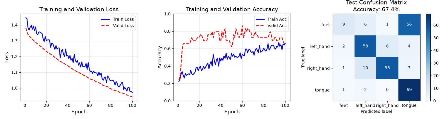
Train Accuracy:    73.96%
Test Accuracy:     67.36%
Test Balanced Acc: 67.36%
Visualizing Results#
fig, axes = plt.subplots(1, 3, figsize=(15, 4))

history = clf.history
epochs = range(1, len(history) + 1)

# Loss
ax1 = axes[0]
ax1.plot(epochs, history[:, "train_loss"], "b-", label="Train Loss", linewidth=2)
ax1.plot(epochs, history[:, "valid_loss"], "r--", label="Valid Loss", linewidth=2)
ax1.set_xlabel("Epoch", fontsize=12)
ax1.set_ylabel("Loss", fontsize=12)
ax1.set_title("Training and Validation Loss", fontsize=14)
ax1.legend(fontsize=10)
ax1.grid(True, alpha=0.3)

# Accuracy
ax2 = axes[1]
ax2.plot(epochs, history[:, "train_acc"], "b-", label="Train Acc", linewidth=2)
ax2.plot(epochs, history[:, "valid_acc"], "r--", label="Valid Acc", linewidth=2)
ax2.set_xlabel("Epoch", fontsize=12)
ax2.set_ylabel("Accuracy", fontsize=12)
ax2.set_title("Training and Validation Accuracy", fontsize=14)
ax2.legend(fontsize=10)
ax2.grid(True, alpha=0.3)
ax2.set_ylim([0, 1])

# Confusion Matrix
ax3 = axes[2]
cm = confusion_matrix(y[test_idx], y_pred_test)
disp = ConfusionMatrixDisplay(confusion_matrix=cm, display_labels=le.classes_)
disp.plot(ax=ax3, cmap="Blues", values_format="d")
ax3.set_title(f"Test Confusion Matrix\nAccuracy: {test_acc * 100:.1f}%", fontsize=14)

plt.tight_layout()
plt.show()
Comparing with Different Configurations#
Let’s compare different EEGSPDNet configurations to understand the impact of hyperparameters.
configs = {
    "Small (k=2, depth=1)": {"bimap_sizes": (2, 1), "n_filters": 4},
    "Medium (k=2, depth=2)": {"bimap_sizes": (2, 2), "n_filters": 4},
    "Large (k=2, depth=3)": {"bimap_sizes": (2, 3), "n_filters": 6},
}

print("\nModel Size Comparison:")
print("-" * 60)
for name, config in configs.items():
    temp_model = EEGSPDNet(n_chans=n_chans, n_outputs=n_outputs, **config)
    n_params = sum(p.numel() for p in temp_model.parameters())
    print(f"{name}: {n_params:,} parameters")
Model Size Comparison:
------------------------------------------------------------
Small (k=2, depth=1): 10,124 parameters
Medium (k=2, depth=2): 8,144 parameters
Large (k=2, depth=3): 15,398 parameters
Summary#
In this tutorial, we demonstrated how to:
Create and configure an EEGSPDNet model
Understand the architecture’s channel-specific processing
Train and evaluate on motor imagery data
Compare different model configurations
EEGSPDNet’s channel-specific convolution allows it to learn independent temporal features for each electrode, which is particularly useful for spatially distributed brain signals.
Total running time of the script: (1 minutes 42.198 seconds)
