spd_learn.modules.BiMap

class spd_learn.modules.BiMap(in_features: int, out_features: int, depthwise: int = 1, parametrized: bool = True, orthogonal_map: Literal['cayley', 'matrix_exp', 'householder'] | None = None, init_method: Literal['kaiming_uniform', 'orthogonal', 'stiefel'] = 'kaiming_uniform', seed: int | None = None, device=None, dtype=None)

Bases: Module

Bilinear Mapping Layer for SPD Matrices.

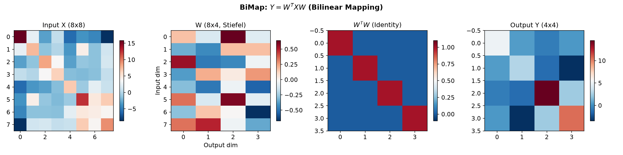
This class implements a bilinear mapping layer for Symmetric Positive Definite (SPD) matrices [Huang and Van Gool, 2017]. The layer transforms an input SPD matrix \(X\) as follows:

\[Y = W^\top X W\]

where \(W \in \mathbb{R}^{n \times k}\) is a learnable weight matrix.

Stiefel Manifold Constraint

When \(W\) has full column rank, the output remains symmetric positive definite. In practice, \(W\) is constrained to the Stiefel manifold \(\text{St}(n, k) = \{W \in \mathbb{R}^{n \times k} : W^\top W = I_k\}\) to preserve geometric structure and numerical stability during training.

Connection to Common Spatial Patterns (CSP)

From an information-geometric perspective, BiMap generalizes Common Spatial Patterns (CSP) [Müller-Gerking et al., 1999] to a learnable setting. CSP learns spatial filters \(W\) from class-wise covariance matrices by maximizing the variance ratio between conditions via a generalized eigenvalue problem:

\[\Sigma^{+} w_i = \lambda_i \Sigma^{-} w_i\]

The subspace spanned by the top-\(k\) CSP filters maximizes the symmetric Kullback-Leibler divergence between Gaussian models of the projected signals. BiMap extends this by learning \(W\) end-to-end within a neural network, allowing adaptation to complex discriminative objectives beyond binary variance ratios.

Parameters:

• in_features (int) – The dimensionality of the input SPD matrices.

• out_features (int) – The dimensionality of the output SPD matrices.

• depthwise (int, default=1) – The number of depthwise bilinear mappings to apply.

• parametrized (bool, default=True) – If True, the weight matrix W is parametrized as an orthogonal matrix via projection/retraction on the Stiefel manifold.

• orthogonal_map ({"cayley", "matrix_exp", "householder"}, optional) – The method used for orthogonal parametrization. If None, defaults to “cayley”.

• init_method ({"kaiming_uniform", "orthogonal", "stiefel"}, default="kaiming_uniform") – The initialization method for the weight matrix.

• seed (int, optional) – The seed for the random number generator used during Stiefel initialization.

Notes

The computational complexity scales as \(O(n^2 k)\) for the bilinear product, making dimensionality reduction (\(k < n\)) beneficial for large covariance matrices.

See also

BiMapIncreaseDim

Bilinear mapping for dimension expansion.

ReEig

Eigenvalue rectification, typically applied after BiMap.

LogEig

Projects to tangent space, typically the final SPD layer.

SPDBatchNormMeanVar

Riemannian batch normalization for SPD matrices.

CovLayer

Computes covariance matrices from time series input.

Examples

>>> import torch
>>> from spd_learn.modules import BiMap
>>> bimap = BiMap(in_features=8, out_features=4)
>>> X = torch.randn(2, 8, 8)
>>> X = X @ X.mT + 0.1 * torch.eye(8)  # Make SPD
>>> Y = bimap(X)
>>> Y.shape
torch.Size([2, 4, 4])

import torch
import numpy as np
import matplotlib.pyplot as plt
from spd_learn.modules import BiMap

torch.manual_seed(42)

# Create an 8x8 SPD matrix
n_in, n_out = 8, 4
A = torch.randn(n_in, n_in)
X = A @ A.T + 0.1 * torch.eye(n_in)
X = X.unsqueeze(0)

# Apply BiMap
bimap = BiMap(in_features=n_in, out_features=n_out, parametrized=True)
Y = bimap(X)

fig, axes = plt.subplots(1, 4, figsize=(16, 4))

# Input
ax1 = axes[0]
im1 = ax1.imshow(X[0].numpy(), cmap='RdBu_r', aspect='auto')
ax1.set_title(f'Input X ({n_in}x{n_in})')
plt.colorbar(im1, ax=ax1, shrink=0.8)

# Weight matrix W
ax2 = axes[1]
W = bimap.weight[0].detach().numpy()
im2 = ax2.imshow(W, cmap='RdBu_r', aspect='auto')
ax2.set_title(f'W ({n_in}x{n_out}, Stiefel)')
ax2.set_xlabel('Output dim')
ax2.set_ylabel('Input dim')
plt.colorbar(im2, ax=ax2, shrink=0.8)

# W^T W (should be identity)
ax3 = axes[2]
WtW = (bimap.weight[0].T @ bimap.weight[0]).detach().numpy()
im3 = ax3.imshow(WtW, cmap='RdBu_r', aspect='auto', vmin=-0.1, vmax=1.1)
ax3.set_title(r'$W^T W$ (Identity)')
plt.colorbar(im3, ax=ax3, shrink=0.8)

# Output
ax4 = axes[3]
im4 = ax4.imshow(Y[0].detach().numpy(), cmap='RdBu_r', aspect='auto')
ax4.set_title(f'Output Y ({n_out}x{n_out})')
plt.colorbar(im4, ax=ax4, shrink=0.8)

plt.suptitle(r'BiMap: $Y = W^T X W$ (Bilinear Mapping)', fontweight='bold')
plt.tight_layout()
plt.show()

(Source code)

forward(X: Tensor) → Tensor

Apply bilinear transformation to input SPD matrices.

Parameters:

X (torch.Tensor) – Input SPD matrices with shape (…, n, n).

Returns:

Transformed SPD matrices with shape (…, k, k).

Return type:

torch.Tensor

reset_parameters() → None

Initialize weight matrix according to the specified method.

weight: Parameter