
Note
Go to the end to download the full example code.
Phase-Space Embedding with PhaseSPDNet#
This tutorial demonstrates how to use PhaseSPDNet for EEG classification. PhaseSPDNet applies phase-space embedding (time-delay coordinates) to capture nonlinear dynamical structure before SPDNet processing.
Introduction#
PhaseSPDNet [Carrara* et al., 2024] leverages phase-space embedding from dynamical systems theory. The key idea is that a single time series can be “unfolded” into a higher-dimensional space that reveals the underlying dynamics of the system.
Takens’ Embedding Theorem: For a dynamical system, a time-delayed embedding can reconstruct the topology of the original state space:
This is particularly useful for EEG, where signals reflect complex brain dynamics that may not be fully captured by linear methods.
Setup and Imports#
import warnings

import matplotlib.pyplot as plt
import numpy as np
import torch

from braindecode import EEGClassifier
from moabb.datasets import BNCI2014_001
from moabb.paradigms import MotorImagery
from sklearn.metrics import ConfusionMatrixDisplay, accuracy_score, confusion_matrix
from sklearn.preprocessing import LabelEncoder
from skorch.callbacks import EpochScoring, GradientNormClipping
from skorch.dataset import ValidSplit

from spd_learn.models import PhaseSPDNet


warnings.filterwarnings("ignore")
/opt/hostedtoolcache/Python/3.11.16/x64/lib/python3.11/site-packages/braindecode/models/eegpt.py:497: FutureWarning: Montage name 'standard_1020' is deprecated and will be removed in MNE 1.14. Use 'colin27_1020' instead.
  montage = mne.channels.make_standard_montage("standard_1020")
/opt/hostedtoolcache/Python/3.11.16/x64/lib/python3.11/site-packages/braindecode/models/eegpt.py:1452: FutureWarning: Montage name 'standard_1020' is deprecated and will be removed in MNE 1.14. Use 'colin27_1020' instead.
  montage = make_standard_montage("standard_1020")
Loading the Dataset#
dataset = BNCI2014_001()
paradigm = MotorImagery(n_classes=4)

print(f"Dataset: {dataset.code}")
print("Sampling rate: 250 Hz")
Choosing from all possible events
Dataset: BNCI2014-001
Sampling rate: 250 Hz
Understanding Phase-Space Embedding#
For a signal with n_chans channels, phase-space embedding with
order=m and lag=τ creates:
This increases the channel dimension by a factor of m:
n_chans → n_chans * order
Choosing parameters:
order: Embedding dimension (typically 2-5)lag: Time delay in samples (often chosen via autocorrelation)
# Visualize embedding concept
fig, axes = plt.subplots(1, 2, figsize=(12, 4))

# Original 1D signal
t = np.linspace(0, 4 * np.pi, 200)
x = np.sin(t) + 0.5 * np.sin(2 * t)

ax1 = axes[0]
ax1.plot(t, x, "b-", linewidth=2)
ax1.set_xlabel("Time", fontsize=12)
ax1.set_ylabel("Amplitude", fontsize=12)
ax1.set_title("Original Signal", fontsize=14)
ax1.grid(True, alpha=0.3)

# Phase-space embedding (2D)
lag = 15  # samples
x_delayed = x[:-lag]
x_original = x[lag:]

ax2 = axes[1]
ax2.plot(x_original, x_delayed, "b-", linewidth=1, alpha=0.7)
ax2.scatter(x_original[::10], x_delayed[::10], c=t[lag::10], cmap="viridis", s=30)
ax2.set_xlabel("x(t)", fontsize=12)
ax2.set_ylabel("x(t - τ)", fontsize=12)
ax2.set_title("Phase-Space Embedding (2D)", fontsize=14)
ax2.grid(True, alpha=0.3)
ax2.set_aspect("equal")

plt.tight_layout()
plt.show()

print("Phase-space embedding reveals the underlying attractor structure!")
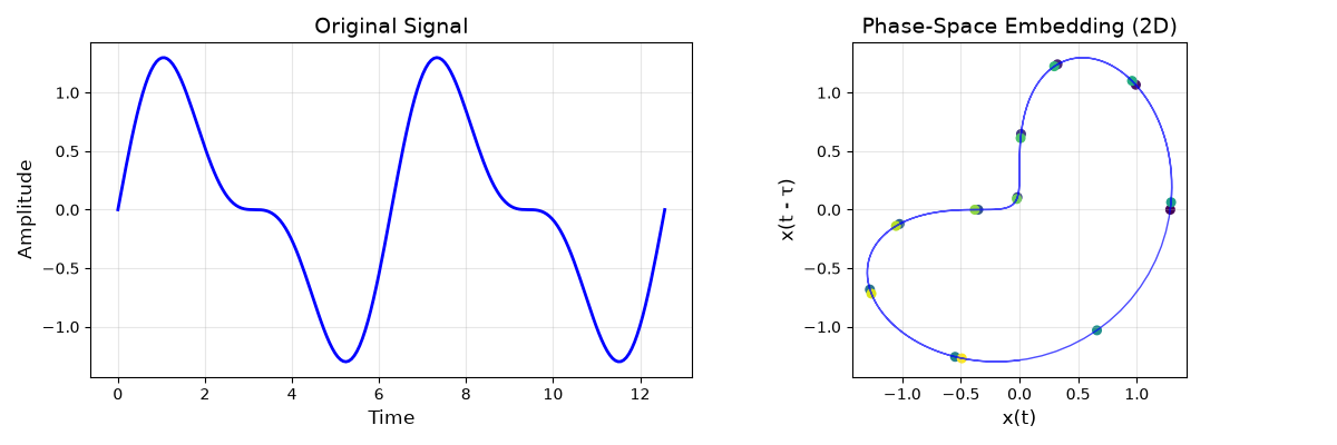
Phase-space embedding reveals the underlying attractor structure!
Creating the PhaseSPDNet Model#
PhaseSPDNet architecture:
PhaseDelay: Applies time-delay embedding
SPDNet: Processes the embedded signals
The embedding expands channels: 22 channels x order 3 = 66 channels
n_chans = 22
n_outputs = 4

# Phase-space parameters
order = 2  # Embedding dimension (lower for stability)
lag = 10  # Time delay (~40ms at 250Hz)

model = PhaseSPDNet(
    n_chans=n_chans,
    n_outputs=n_outputs,
    order=order,
    lag=lag,
    subspacedim=22,  # BiMap output dimension (half of embedded channels)
    threshold=1e-4,
)

print("PhaseSPDNet Configuration:")
print(f"  Original channels: {n_chans}")
print(f"  Embedding order: {order}")
print(f"  Time lag: {lag} samples ({lag / 250 * 1000:.1f} ms)")
print(f"  Embedded channels: {n_chans * order}")
print("  Subspace dimension: 22")
print("\nModel Architecture:")
print(model)
PhaseSPDNet Configuration:
  Original channels: 22
  Embedding order: 2
  Time lag: 10 samples (40.0 ms)
  Embedded channels: 44
  Subspace dimension: 22

Model Architecture:
PhaseSPDNet(
  (phase): PhaseDelay()
  (spdnet): SPDNet(
    (cov): CovLayer()
    (bimap): ParametrizedBiMap(
      (parametrizations): ModuleDict(
        (weight): ParametrizationList(
          (0): _Orthogonal()
        )
      )
    )
    (reeig): ReEig()
    (logeig): LogEig()
    (classifier): Linear(in_features=253, out_features=4, bias=True)
  )
)
Training the Model#
subject_id = 1
batch_size = 32
max_epochs = 100
learning_rate = 1e-4  # Low learning rate for stable SPD learning

device = "cuda" if torch.cuda.is_available() else "cpu"
print(f"\nUsing device: {device}")

# Cache configuration
cache_config = dict(
    save_raw=True,
    save_epochs=True,
    save_array=True,
    use=True,
    overwrite_raw=False,
    overwrite_epochs=False,
    overwrite_array=False,
)

# Load data
X, labels, meta = paradigm.get_data(
    dataset=dataset, subjects=[subject_id], cache_config=cache_config
)

# Encode labels
le = LabelEncoder()
y = le.fit_transform(labels)

# Split by session
train_idx = meta.query("session == '0train'").index.to_numpy()
test_idx = meta.query("session == '1test'").index.to_numpy()

print(f"\nData shape: {X.shape}")
print(
    f"After embedding: ({X.shape[0]}, {n_chans * order}, {X.shape[2] - (order - 1) * lag})"
)
print(f"Training samples: {len(train_idx)}")
print(f"Test samples: {len(test_idx)}")

# Create classifier
# Note: SPD networks benefit from gradient clipping to prevent
# divergence during training on the Riemannian manifold.
clf = EEGClassifier(
    model,
    criterion=torch.nn.CrossEntropyLoss,
    optimizer=torch.optim.Adam,
    optimizer__lr=learning_rate,
    train_split=ValidSplit(0.1, stratified=True, random_state=42),
    batch_size=batch_size,
    max_epochs=max_epochs,
    callbacks=[
        (
            "train_acc",
            EpochScoring(
                "accuracy", lower_is_better=False, on_train=True, name="train_acc"
            ),
        ),
        ("gradient_clip", GradientNormClipping(gradient_clip_value=1.0)),
    ],
    device=device,
    verbose=1,
)

# Train
clf.fit(X[train_idx], y[train_idx])

# Evaluate
y_pred_train = clf.predict(X[train_idx])
y_pred_test = clf.predict(X[test_idx])

train_acc = accuracy_score(y[train_idx], y_pred_train)
test_acc = accuracy_score(y[test_idx], y_pred_test)

print(f"\n{'=' * 50}")
print(f"Results for Subject {subject_id}")
print(f"{'=' * 50}")
print(f"Train Accuracy: {train_acc * 100:.2f}%")
print(f"Test Accuracy:  {test_acc * 100:.2f}%")
Using device: cpu

Data shape: (576, 22, 1001)
After embedding: (576, 44, 991)
Training samples: 288
Test samples: 288
  epoch    train_acc    train_loss    valid_acc    valid_loss     dur
-------  -----------  ------------  -----------  ------------  ------
      1       0.3242        1.4330       0.4138        1.3895  0.1477
      2       0.3750        1.4028       0.4828        1.3713  0.1400
      3       0.3750        1.3809       0.3793        1.3607  0.1537
      4       0.3125        1.3715       0.3103        1.3542  0.1549
      5       0.3164        1.3656       0.3103        1.3502  0.1427
      6       0.3594        1.3558       0.2759        1.3445  0.1417
      7       0.3555        1.3513       0.3448        1.3397  0.1380
      8       0.3750        1.3446       0.3448        1.3337  0.1386
      9       0.3789        1.3382       0.3103        1.3268  0.1510
     10       0.3633        1.3327       0.3448        1.3211  0.1558
     11       0.3789        1.3266       0.3448        1.3148  0.1521
     12       0.4023        1.3205       0.3103        1.3093  0.1392
     13       0.4141        1.3155       0.4138        1.3036  0.1408
     14       0.4102        1.3106       0.3793        1.2982  0.1420
     15       0.4102        1.3046       0.3793        1.2928  0.1414
     16       0.4414        1.2993       0.3793        1.2864  0.1591
     17       0.4688        1.2935       0.3793        1.2812  0.1462
     18       0.4844        1.2887       0.4483        1.2771  0.1392
     19       0.5195        1.2831       0.5172        1.2728  0.1391
     20       0.5547        1.2774       0.5172        1.2677  0.1369
     21       0.5508        1.2735       0.4483        1.2632  0.1426
     22       0.5273        1.2680       0.4138        1.2566  0.1592
     23       0.5391        1.2650       0.4138        1.2523  0.1565
     24       0.5430        1.2555       0.4138        1.2474  0.1412
     25       0.5430        1.2526       0.4138        1.2427  0.1378
     26       0.5234        1.2469       0.4138        1.2383  0.1370
     27       0.5664        1.2425       0.4138        1.2333  0.1405
     28       0.5820        1.2375       0.4483        1.2280  0.1570
     29       0.5820        1.2326       0.5172        1.2221  0.1555
     30       0.6250        1.2266       0.5172        1.2175  0.1428
     31       0.6602        1.2240       0.5517        1.2138  0.1397
     32       0.6602        1.2190       0.5172        1.2107  0.1431
     33       0.6094        1.2149       0.4483        1.2082  0.1371
     34       0.5938        1.2118       0.4828        1.2056  0.1538
     35       0.6016        1.2072       0.4828        1.2004  0.1563
     36       0.6289        1.2023       0.4483        1.1949  0.1463
     37       0.6484        1.1988       0.5862        1.1891  0.1399
     38       0.6641        1.1945       0.6207        1.1842  0.1424
     39       0.6562        1.1920       0.6207        1.1808  0.1419
     40       0.6289        1.1866       0.5172        1.1781  0.1460
     41       0.6523        1.1829       0.5862        1.1745  0.1579
     42       0.6680        1.1798       0.5862        1.1708  0.1542
     43       0.6914        1.1726       0.5862        1.1665  0.1376
     44       0.6797        1.1658       0.5172        1.1634  0.1384
     45       0.6523        1.1636       0.5172        1.1589  0.1442
     46       0.6602        1.1613       0.5517        1.1539  0.1406
     47       0.6406        1.1570       0.5517        1.1501  0.1548
     48       0.6523        1.1486       0.5517        1.1443  0.1402
     49       0.6797        1.1465       0.5172        1.1392  0.1555
     50       0.6953        1.1412       0.5862        1.1362  0.1503
     51       0.7031        1.1367       0.6897        1.1329  0.1404
     52       0.7109        1.1330       0.6897        1.1283  0.1412
     53       0.6914        1.1307       0.5862        1.1247  0.1413
     54       0.6914        1.1265       0.5862        1.1201  0.1379
     55       0.6836        1.1218       0.5517        1.1159  0.1554
     56       0.6758        1.1175       0.5862        1.1140  0.1577
     57       0.6953        1.1152       0.6207        1.1088  0.1393
     58       0.7305        1.1107       0.6897        1.1054  0.1385
     59       0.7539        1.1070       0.6897        1.1032  0.1445
     60       0.7305        1.1052       0.5862        1.1011  0.1400
     61       0.7109        1.1007       0.5862        1.0984  0.1501
     62       0.7227        1.0972       0.6552        1.0931  0.1520
     63       0.7188        1.0924       0.6207        1.0878  0.1423
     64       0.7070        1.0896       0.6207        1.0847  0.1422
     65       0.7031        1.0844       0.5862        1.0823  0.1406
     66       0.7148        1.0815       0.6207        1.0775  0.1430
     67       0.7344        1.0781       0.6552        1.0730  0.1541
     68       0.7383        1.0750       0.5862        1.0710  0.1507
     69       0.7148        1.0696       0.6207        1.0680  0.1479
     70       0.7148        1.0677       0.6207        1.0655  0.1415
     71       0.7344        1.0645       0.6552        1.0624  0.1405
     72       0.7539        1.0606       0.6897        1.0593  0.1415
     73       0.7695        1.0588       0.7241        1.0545  0.1457
     74       0.7812        1.0563       0.7241        1.0511  0.1617
     75       0.7930        1.0525       0.7586        1.0475  0.1506
     76       0.8125        1.0484       0.7586        1.0434  0.1439
     77       0.8086        1.0451       0.7241        1.0400  0.1401
     78       0.7930        1.0418       0.7241        1.0378  0.1380
     79       0.7656        1.0378       0.7586        1.0360  0.1439
     80       0.7539        1.0344       0.6552        1.0335  0.1564
     81       0.7344        1.0330       0.6552        1.0310  0.1549
     82       0.7305        1.0296       0.7241        1.0271  0.1412
     83       0.7891        1.0271       0.7586        1.0224  0.1400
     84       0.7812        1.0216       0.7241        1.0205  0.1398
     85       0.7617        1.0176       0.6552        1.0192  0.1394
     86       0.7734        1.0140       0.7241        1.0157  0.1548
     87       0.7891        1.0125       0.7586        1.0111  0.1574
     88       0.7773        1.0083       0.7586        1.0088  0.1392
     89       0.7891        1.0049       0.7586        1.0051  0.1391
     90       0.7891        1.0016       0.7241        1.0026  0.1378
     91       0.7617        0.9971       0.6552        1.0027  0.1379
     92       0.7266        0.9957       0.6207        1.0000  0.1532
     93       0.7305        0.9915       0.6552        0.9944  0.1536
     94       0.7695        0.9893       0.7241        0.9897  0.1459
     95       0.8086        0.9867       0.7586        0.9873  0.1381
     96       0.8086        0.9829       0.8276        0.9852  0.1403
     97       0.8086        0.9813       0.7931        0.9832  0.1403
     98       0.8047        0.9776       0.7931        0.9810  0.1491
     99       0.7930        0.9757       0.7586        0.9807  0.1421
    100       0.8047        0.9706       0.7586        0.9772  0.1498

==================================================
Results for Subject 1
==================================================
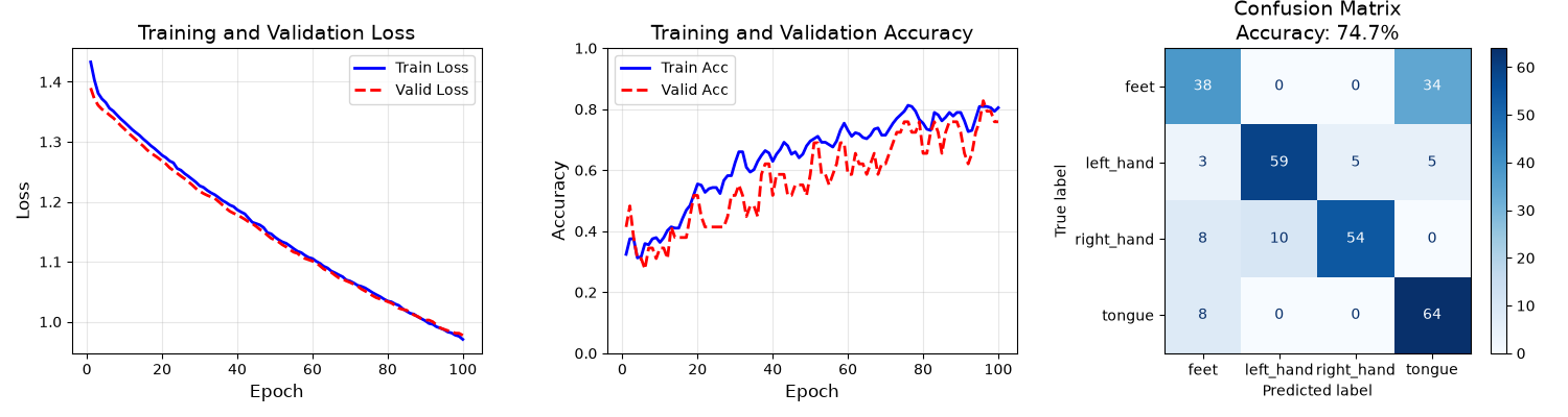
Train Accuracy: 79.51%
Test Accuracy:  74.65%
Visualizing Results#
fig, axes = plt.subplots(1, 3, figsize=(15, 4))

# Training curves
history = clf.history
epochs = range(1, len(history) + 1)

ax1 = axes[0]
ax1.plot(epochs, history[:, "train_loss"], "b-", label="Train Loss", linewidth=2)
ax1.plot(epochs, history[:, "valid_loss"], "r--", label="Valid Loss", linewidth=2)
ax1.set_xlabel("Epoch", fontsize=12)
ax1.set_ylabel("Loss", fontsize=12)
ax1.set_title("Training and Validation Loss", fontsize=14)
ax1.legend(fontsize=10)
ax1.grid(True, alpha=0.3)

ax2 = axes[1]
ax2.plot(epochs, history[:, "train_acc"], "b-", label="Train Acc", linewidth=2)
ax2.plot(epochs, history[:, "valid_acc"], "r--", label="Valid Acc", linewidth=2)
ax2.set_xlabel("Epoch", fontsize=12)
ax2.set_ylabel("Accuracy", fontsize=12)
ax2.set_title("Training and Validation Accuracy", fontsize=14)
ax2.legend(fontsize=10)
ax2.grid(True, alpha=0.3)
ax2.set_ylim([0, 1])

# Confusion matrix
ax3 = axes[2]
cm = confusion_matrix(y[test_idx], y_pred_test)
disp = ConfusionMatrixDisplay(confusion_matrix=cm, display_labels=le.classes_)
disp.plot(ax=ax3, cmap="Blues", values_format="d")
ax3.set_title(f"Confusion Matrix\nAccuracy: {test_acc * 100:.1f}%", fontsize=14)

plt.tight_layout()
plt.show()
Comparing Different Embedding Parameters#
The choice of order and lag affects performance.
Let’s compare different configurations.
print("\nComparing embedding parameters:")
print("-" * 50)

configs = [
    {"order": 2, "lag": 5, "name": "order=2, lag=5"},
    {"order": 2, "lag": 10, "name": "order=2, lag=10"},
    {"order": 3, "lag": 5, "name": "order=3, lag=5"},
    {"order": 3, "lag": 10, "name": "order=3, lag=10"},
]

for config in configs:
    embedded_chans = n_chans * config["order"]
    reduced_time = X.shape[2] - (config["order"] - 1) * config["lag"]
    cov_size = embedded_chans * (embedded_chans + 1) // 2
    print(
        f"{config['name']:20s}: {embedded_chans} channels, "
        f"{reduced_time} time points, {cov_size} features"
    )
Comparing embedding parameters:
--------------------------------------------------
order=2, lag=5      : 44 channels, 996 time points, 990 features
order=2, lag=10     : 44 channels, 991 time points, 990 features
order=3, lag=5      : 66 channels, 991 time points, 2211 features
order=3, lag=10     : 66 channels, 981 time points, 2211 features
When to Use Phase-Space Embedding#
PhaseSPDNet is particularly effective when:
Nonlinear dynamics: The underlying system has complex, nonlinear behavior (e.g., neural oscillations, chaos)
Limited channels: Embedding can extract more information from fewer channels
Temporal structure: Important features span across time (captured by delay coordinates)
Considerations:
Higher
orderincreases model capacity but also parameterslagshould be chosen based on the signal’s autocorrelationReduces effective time dimension:
T_new = T - (order-1) * lag
Summary#
In this tutorial, we demonstrated:
Phase-space embedding theory and visualization
Creating PhaseSPDNet with different embedding parameters
Training and evaluating on motor imagery data
PhaseSPDNet offers a principled way to incorporate dynamical systems perspectives into EEG classification, potentially capturing nonlinear brain dynamics that linear methods miss.
Total running time of the script: (0 minutes 21.184 seconds)
