
Note
Go to the end to download the full example code.
Cross-Session Transfer with TSMNet#
This tutorial demonstrates how to use TSMNet for cross-session motor imagery classification with domain adaptation. TSMNet’s SPDBatchNormMeanVar layer enables adaptation to new sessions without labeled data from the target session.
Introduction#
In EEG-based BCIs, a common challenge is session-to-session variability: models trained on one day often perform poorly on another day due to changes in electrode impedance, mental state, and environment.
TSMNet [Kobler et al., 2022] addresses this through SPDBatchNormMeanVar, which:
Normalizes SPD matrices using the Fréchet mean
Maintains running statistics that can be updated on new data
Enables Source-Free Unsupervised Domain Adaptation (SFUDA)
This means we can adapt to a new subject using only unlabeled data!
Setup and Imports#
import warnings

from typing import List, Tuple

import matplotlib.pyplot as plt
import numpy as np
import torch

from braindecode import EEGClassifier
from moabb.datasets import BNCI2014_001
from moabb.paradigms import MotorImagery
from skada import (
    CORALAdapter,
    EntropicOTMapping,
    SubspaceAlignment,
    make_da_pipeline,
)
from sklearn.decomposition import PCA
from sklearn.linear_model import LogisticRegression
from sklearn.metrics import accuracy_score
from sklearn.preprocessing import LabelEncoder, StandardScaler
from skorch.callbacks import EpochScoring, GradientNormClipping
from skorch.dataset import ValidSplit

from spd_learn.models import TSMNet


warnings.filterwarnings("ignore")
/opt/hostedtoolcache/Python/3.11.16/x64/lib/python3.11/site-packages/braindecode/models/eegpt.py:497: FutureWarning: Montage name 'standard_1020' is deprecated and will be removed in MNE 1.14. Use 'colin27_1020' instead.
  montage = mne.channels.make_standard_montage("standard_1020")
/opt/hostedtoolcache/Python/3.11.16/x64/lib/python3.11/site-packages/braindecode/models/eegpt.py:1452: FutureWarning: Montage name 'standard_1020' is deprecated and will be removed in MNE 1.14. Use 'colin27_1020' instead.
  montage = make_standard_montage("standard_1020")
Loading the Dataset#
BNCI2014_001 contains EEG recordings from 9 subjects performing - 22 EEG channels: Standard 10-20 montage - 250 Hz sampling rate: After resampling
We’ll demonstrate cross-session transfer:
Source domain: Subject 1, Session 1 (training)
Target domain: Subject 1, Session 2 (testing/adaptation)
Cross-session transfer is a realistic BCI scenario where we want to avoid recalibration for a returning user.
dataset = BNCI2014_001()
paradigm = MotorImagery(n_classes=4)

print(f"Dataset: {dataset.code}")
print("Cross-subject transfer: Subject 1 (source) -> Subject 2 (target)")
Choosing from all possible events
Dataset: BNCI2014-001
Cross-subject transfer: Subject 1 (source) -> Subject 2 (target)
Creating the TSMNet Model#
TSMNet architecture:
Temporal Conv: Learns temporal filters
Spatial Conv: Learns spatial combinations
CovLayer: Computes covariance matrices
BiMap + ReEig: SPD dimensionality reduction
SPDBatchNormMeanVar: Riemannian batch normalization (key for adaptation)
LogEig: Projects to tangent space
Linear: Classification head
n_chans = 22
n_outputs = 4

model = TSMNet(
    n_chans=n_chans,
    n_outputs=n_outputs,
    n_temp_filters=8,  # Temporal filters
    temp_kernel_length=50,  # ~200ms at 250Hz
    n_spatiotemp_filters=32,  # Spatiotemporal features
    n_bimap_filters=16,  # BiMap output dimension
    reeig_threshold=1e-4,  # ReEig threshold
)

print("TSMNet Architecture:")
print(model)
TSMNet Architecture:
TSMNet(
  (cnn): Sequential(
    (0): Conv2d(1, 8, kernel_size=(1, 50), stride=(1, 1), padding=same, padding_mode=reflect)
    (1): Conv2d(8, 32, kernel_size=(22, 1), stride=(1, 1))
    (2): Flatten(start_dim=2, end_dim=-1)
  )
  (covpool): CovLayer()
  (spdnet): Sequential(
    (0): ParametrizedBiMap(
      (parametrizations): ModuleDict(
        (weight): ParametrizationList(
          (0): _Orthogonal()
        )
      )
    )
    (1): ReEig()
  )
  (spdbnorm): ParametrizedSPDBatchNormMeanVar(
    (parametrizations): ModuleDict(
      (weight): ParametrizationList(
        (0): PositiveDefiniteScalar()
      )
      (bias): ParametrizationList(
        (0): SymmetricPositiveDefinite()
      )
    )
  )
  (logeig): Sequential(
    (0): LogEig()
    (1): Flatten(start_dim=1, end_dim=-1)
  )
  (head): Linear(in_features=136, out_features=4, bias=True)
)
Training on Source Domain#
First, we train TSMNet on Session 1 (source domain).
source_subject = 1
target_subject = 1  # Same subject, different session
batch_size = 32
max_epochs = 300
learning_rate = 1e-4  # Optimal learning rate from grid search
weight_decay = 1e-4  # L2 regularization for better generalization

device = "cuda" if torch.cuda.is_available() else "cpu"
print(f"\nUsing device: {device}")

# Cache configuration
cache_config = dict(
    save_raw=True,
    save_epochs=True,
    save_array=True,
    use=True,
    overwrite_raw=False,
    overwrite_epochs=False,
    overwrite_array=False,
)

# Load data for both subjects
X, labels, meta = paradigm.get_data(
    dataset=dataset,
    subjects=[source_subject, target_subject],
    cache_config=cache_config,
)

# Encode labels
le = LabelEncoder()
y = le.fit_transform(labels)

# Split by session
# Session '0train' is the first session (source)
# Session '1test' is the second session (target)
source_idx = meta.query("session == '0train'").index.to_numpy()
target_idx = meta.query("session == '1test'").index.to_numpy()

X_source, y_source = X[source_idx], y[source_idx]
X_target, y_target = X[target_idx], y[target_idx]

print(f"\nSource domain (Session 1): {len(source_idx)} samples")
print(f"Target domain (Session 2): {len(target_idx)} samples")

# Create classifier
# Note: SPD networks benefit from gradient clipping to prevent
# divergence during training on the Riemannian manifold.
clf = EEGClassifier(
    model,
    criterion=torch.nn.CrossEntropyLoss,
    optimizer=torch.optim.AdamW,
    optimizer__lr=learning_rate,
    optimizer__weight_decay=weight_decay,
    train_split=ValidSplit(0.1, stratified=True, random_state=42),
    batch_size=batch_size,
    max_epochs=max_epochs,
    callbacks=[
        (
            "train_acc",
            EpochScoring(
                "accuracy", lower_is_better=False, on_train=True, name="train_acc"
            ),
        ),
        ("gradient_clip", GradientNormClipping(gradient_clip_value=1.0)),
    ],
    device=device,
    verbose=1,
)

# Train on source domain
print("\n" + "=" * 50)
print("Training on Source Domain")
print("=" * 50)
clf.fit(X_source, y_source)
Using device: cpu
Source domain (Session 1): 288 samples
Target domain (Session 2): 288 samples
==================================================
Training on Source Domain
==================================================
epoch train_acc train_loss valid_acc valid_loss dur
------- ----------- ------------ ----------- ------------ ------
1 0.1914 1.3997 0.1034 1.3837 1.4583
2 0.3047 1.3880 0.3793 1.3665 1.4320
3 0.3750 1.3778 0.4483 1.3560 1.4156
4 0.4102 1.3685 0.4828 1.3459 1.4367
5 0.4570 1.3580 0.4828 1.3387 1.4078
6 0.4727 1.3508 0.5172 1.3315 1.4286
7 0.4688 1.3414 0.4138 1.3258 1.4060
8 0.4727 1.3360 0.4483 1.3196 1.4451
9 0.4766 1.3264 0.5172 1.3134 1.4083
10 0.4727 1.3230 0.4828 1.3095 1.4312
11 0.4766 1.3180 0.5172 1.3043 1.4133
12 0.4766 1.3125 0.5172 1.2995 1.4254
13 0.4883 1.3061 0.4828 1.2952 1.4274
14 0.4805 1.3028 0.5172 1.2897 1.4418
15 0.4727 1.2981 0.5172 1.2844 1.4435
16 0.4844 1.2908 0.5172 1.2802 1.4399
17 0.4766 1.2875 0.5172 1.2756 1.4513
18 0.4844 1.2831 0.5172 1.2704 1.4418
19 0.4883 1.2781 0.5172 1.2663 1.4387
20 0.4922 1.2748 0.5172 1.2617 1.4319
21 0.5039 1.2688 0.5172 1.2571 1.4437
22 0.4961 1.2639 0.5172 1.2533 1.2783
23 0.5078 1.2592 0.5172 1.2491 1.3794
24 0.5000 1.2584 0.5172 1.2448 1.4444
25 0.5000 1.2552 0.4828 1.2422 1.3413
26 0.5039 1.2477 0.4828 1.2372 0.9242
27 0.5156 1.2477 0.5172 1.2325 0.9394
28 0.5234 1.2426 0.4828 1.2287 0.9033
29 0.5195 1.2366 0.5172 1.2246 0.9515
30 0.5352 1.2321 0.4828 1.2223 0.8935
31 0.5312 1.2340 0.5172 1.2182 0.9175
32 0.5273 1.2250 0.5172 1.2144 0.8910
33 0.5312 1.2270 0.5172 1.2103 0.8836
34 0.5352 1.2185 0.5172 1.2064 0.9082
35 0.5391 1.2142 0.5172 1.2033 0.9079
36 0.5352 1.2090 0.5172 1.1990 0.9189
37 0.5391 1.2049 0.4828 1.1949 0.8910
38 0.5430 1.2130 0.4828 1.1926 0.8902
39 0.5508 1.1989 0.4828 1.1870 0.9267
40 0.5391 1.1962 0.4828 1.1835 0.8884
41 0.5430 1.1955 0.4828 1.1804 0.8884
42 0.5586 1.1906 0.5172 1.1772 0.8928
43 0.5625 1.1846 0.4828 1.1736 0.8907
44 0.5547 1.1819 0.4828 1.1696 0.8849
45 0.5586 1.1804 0.4828 1.1670 0.8892
46 0.5703 1.1746 0.4828 1.1636 0.8852
47 0.5625 1.1749 0.5517 1.1609 0.8887
48 0.5625 1.1747 0.4828 1.1574 0.9040
49 0.5820 1.1639 0.4828 1.1564 0.8922
50 0.5586 1.1648 0.4828 1.1508 0.9130
51 0.5703 1.1684 0.5172 1.1465 0.9194
52 0.5820 1.1606 0.5172 1.1459 0.9016
53 0.5820 1.1520 0.5172 1.1440 0.9265
54 0.5859 1.1521 0.5172 1.1398 0.9362
55 0.6094 1.1458 0.4828 1.1343 0.9166
56 0.5977 1.1455 0.4828 1.1301 0.8798
57 0.5820 1.1408 0.4828 1.1281 0.8942
58 0.5820 1.1453 0.5172 1.1253 0.8808
59 0.6094 1.1310 0.4828 1.1212 0.8938
60 0.6133 1.1306 0.4828 1.1174 0.8828
61 0.5898 1.1287 0.5517 1.1163 0.8944
62 0.5859 1.1331 0.4828 1.1140 0.8932
63 0.5977 1.1219 0.4828 1.1087 0.8886
64 0.5977 1.1262 0.5172 1.1059 0.8746
65 0.6172 1.1178 0.4828 1.1032 0.8842
66 0.6055 1.1206 0.5517 1.1027 0.8824
67 0.6055 1.1159 0.5517 1.0970 0.8863
68 0.6094 1.1074 0.4828 1.0965 0.8865
69 0.6250 1.1093 0.4828 1.0970 0.8869
70 0.6172 1.1051 0.5517 1.0913 0.8899
71 0.6328 1.1078 0.4828 1.0928 0.8822
72 0.6172 1.1134 0.5172 1.0865 0.8841
73 0.6328 1.1033 0.4828 1.0835 0.8847
74 0.6289 1.0999 0.5172 1.0801 0.9162
75 0.6250 1.0936 0.4828 1.0765 0.9249
76 0.6250 1.0962 0.5172 1.0745 0.9058
77 0.6367 1.0879 0.5517 1.0757 0.8856
78 0.6328 1.0898 0.5517 1.0718 0.8782
79 0.6328 1.0846 0.5517 1.0683 0.8894
80 0.6289 1.0855 0.4828 1.0677 0.8771
81 0.6289 1.0817 0.5172 1.0724 0.8838
82 0.6484 1.0794 0.5172 1.0741 0.8895
83 0.6328 1.0794 0.5172 1.0735 0.8972
84 0.6406 1.0764 0.5172 1.0682 0.8865
85 0.6328 1.0849 0.5172 1.0588 0.8865
86 0.6484 1.0688 0.5517 1.0521 0.8903
87 0.6406 1.0752 0.5517 1.0499 0.8982
88 0.6641 1.0662 0.5517 1.0497 0.8908
89 0.6523 1.0629 0.5517 1.0469 0.8905
90 0.6523 1.0591 0.5172 1.0484 0.8855
91 0.6484 1.0584 0.5172 1.0465 0.8916
92 0.6484 1.0524 0.5517 1.0407 0.8787
93 0.6523 1.0544 0.5517 1.0397 0.8847
94 0.6250 1.0564 0.4828 1.0398 0.8888
95 0.6484 1.0547 0.5517 1.0335 0.8902
96 0.6406 1.0568 0.5517 1.0356 0.8866
97 0.6406 1.0494 0.5517 1.0343 0.8904
98 0.6602 1.0420 0.5517 1.0291 1.3483
99 0.6445 1.0437 0.5172 1.0263 0.9137
100 0.6445 1.0446 0.5172 1.0322 0.8855
101 0.6562 1.0328 0.4828 1.0260 0.8877
102 0.6641 1.0344 0.5517 1.0206 0.8799
103 0.6602 1.0316 0.5172 1.0202 0.8790
104 0.6562 1.0288 0.5517 1.0205 0.8791
105 0.6523 1.0326 0.5517 1.0172 0.8737
106 0.6523 1.0274 0.5517 1.0122 0.8868
107 0.6523 1.0326 0.5517 1.0117 0.8758
108 0.6445 1.0339 0.5172 1.0073 0.8796
109 0.6602 1.0227 0.5172 1.0082 0.8889
110 0.6641 1.0212 0.5172 1.0081 0.8974
111 0.6641 1.0199 0.4828 1.0083 0.9452
112 0.6523 1.0261 0.5172 1.0065 0.8834
113 0.6680 1.0170 0.5517 1.0011 0.8912
114 0.6797 1.0089 0.5172 1.0031 0.8958
115 0.6641 1.0188 0.4828 1.0039 0.8891
116 0.6719 1.0130 0.5862 1.0022 0.8869
117 0.6562 1.0130 0.5172 1.0061 0.8886
118 0.6641 1.0122 0.5517 0.9989 0.8910
119 0.6797 1.0001 0.5517 0.9957 0.8809
120 0.6680 1.0022 0.5517 1.0027 0.8945
121 0.6719 0.9984 0.5517 0.9953 0.8906
122 0.6602 1.0031 0.5517 0.9970 0.8881
123 0.6680 1.0012 0.5517 0.9879 0.8996
124 0.6680 0.9975 0.5517 0.9877 0.8938
125 0.6641 0.9961 0.5862 0.9864 0.8911
126 0.6719 0.9919 0.5172 0.9930 0.8818
127 0.6406 0.9973 0.5172 0.9874 0.8888
128 0.6914 0.9854 0.5862 0.9822 0.8891
129 0.6602 0.9936 0.5517 0.9788 0.9155
130 0.6680 0.9868 0.5517 0.9770 0.9580
131 0.6797 0.9844 0.4828 0.9861 1.1718
132 0.6602 0.9870 0.5172 0.9793 1.3062
133 0.6797 0.9734 0.5172 0.9746 0.8834
134 0.6641 0.9858 0.5517 0.9708 1.2690
135 0.6562 0.9976 0.5172 0.9691 1.4022
136 0.6602 0.9827 0.5517 0.9753 1.3208
137 0.6836 0.9693 0.5862 0.9728 1.1920
138 0.6797 0.9744 0.5172 0.9812 1.2029
139 0.6680 0.9788 0.5172 0.9672 1.2865
140 0.6641 0.9834 0.5862 0.9712 1.4385
141 0.6680 0.9721 0.5862 0.9695 0.8953
142 0.6680 0.9772 0.5517 0.9620 0.8913
143 0.6562 0.9675 0.5172 0.9628 1.2394
144 0.6836 0.9686 0.5172 0.9584 0.8890
145 0.6797 0.9654 0.5517 0.9588 1.2748
146 0.6680 0.9631 0.5517 0.9601 0.9037
147 0.6914 0.9584 0.5862 0.9622 1.1323
148 0.6719 0.9646 0.5862 0.9633 1.1696
149 0.6875 0.9600 0.5862 0.9570 1.2156
150 0.6641 0.9580 0.5172 0.9584 1.0080
151 0.6602 0.9641 0.5862 0.9565 1.4063
152 0.6875 0.9618 0.5862 0.9528 1.0643
153 0.6523 0.9610 0.5862 0.9513 0.8794
154 0.6797 0.9467 0.5862 0.9484 0.8864
155 0.6641 0.9622 0.5517 0.9474 0.8946
156 0.6680 0.9517 0.4828 0.9516 0.8912
157 0.6680 0.9472 0.5517 0.9590 1.1167
158 0.6914 0.9454 0.6207 0.9516 0.9824
159 0.6953 0.9456 0.4828 0.9474 1.1984
160 0.6758 0.9402 0.5517 0.9387 1.4206
161 0.6719 0.9498 0.5172 0.9510 1.4101
162 0.6680 0.9517 0.5172 0.9522 0.8875
163 0.6758 0.9370 0.5862 0.9438 0.8865
164 0.6797 0.9387 0.4828 0.9452 0.8898
165 0.6953 0.9265 0.5862 0.9402 0.8869
166 0.6953 0.9330 0.4828 0.9492 0.8913
167 0.6914 0.9306 0.5862 0.9463 0.8887
168 0.6641 0.9399 0.4828 0.9593 0.8917
169 0.6719 0.9264 0.5862 0.9372 0.8975
170 0.6953 0.9290 0.5862 0.9366 0.8899
171 0.6992 0.9178 0.6207 0.9352 0.8819
172 0.6914 0.9264 0.5862 0.9256 0.8899
173 0.6914 0.9305 0.5172 0.9370 0.8871
174 0.7031 0.9222 0.4828 0.9536 0.9042
175 0.6953 0.9201 0.5862 0.9262 0.8966
176 0.6680 0.9233 0.5862 0.9277 0.8914
177 0.6914 0.9221 0.5517 0.9264 0.8926
178 0.6875 0.9152 0.5862 0.9228 0.8904
179 0.6875 0.9180 0.5862 0.9254 0.8946
180 0.6875 0.9211 0.5172 0.9352 0.8956
181 0.7070 0.9164 0.4828 0.9326 0.8952
182 0.6719 0.9109 0.5172 0.9413 0.8972
183 0.6836 0.9195 0.5517 0.9188 0.8925
184 0.6836 0.9112 0.5862 0.9233 0.8994
185 0.6875 0.9110 0.6207 0.9252 0.8977
186 0.6914 0.9146 0.6552 0.9249 0.8879
187 0.6680 0.9196 0.5862 0.9274 0.8948
188 0.6875 0.9113 0.5862 0.9226 0.8898
189 0.6836 0.9151 0.5862 0.9131 0.9020
190 0.7031 0.8971 0.5862 0.9101 0.8950
191 0.6914 0.8978 0.5862 0.9127 0.8965
192 0.6875 0.9137 0.5517 0.9085 0.8989
193 0.7031 0.9095 0.5862 0.9065 0.8937
194 0.6953 0.9030 0.4828 0.9196 0.8978
195 0.6953 0.8921 0.5517 0.9096 0.8985
196 0.6953 0.8938 0.5862 0.9085 0.8933
197 0.6914 0.9043 0.5862 0.9072 0.8916
198 0.6914 0.9064 0.5862 0.9075 0.8969
199 0.6719 0.8961 0.5862 0.9047 0.8973
200 0.7031 0.8900 0.5862 0.9035 0.9064
201 0.7070 0.8932 0.5862 0.9070 0.9194
202 0.6914 0.9055 0.5517 0.9090 0.9325
203 0.6953 0.9074 0.6207 0.9084 0.9004
204 0.7070 0.8856 0.5517 0.9182 0.8984
205 0.6875 0.8855 0.4828 0.9313 0.8958
206 0.7031 0.8838 0.4828 0.9252 0.8956
207 0.6953 0.8900 0.5172 0.9223 0.8961
208 0.6953 0.8935 0.5862 0.8996 0.8994
209 0.6953 0.8845 0.5862 0.9004 0.9050
210 0.6914 0.8761 0.5862 0.9007 0.8879
211 0.6797 0.8946 0.5862 0.8941 0.8888
212 0.7031 0.8881 0.5862 0.8930 0.8920
213 0.7148 0.8731 0.5862 0.8985 0.9005
214 0.6914 0.8767 0.5862 0.8985 0.9062
215 0.6953 0.8746 0.5862 0.9046 0.8893
216 0.7148 0.8693 0.5862 0.8980 0.9010
217 0.7031 0.8753 0.5862 0.8924 0.8917
218 0.7070 0.8762 0.5862 0.8929 0.8924
219 0.7109 0.8671 0.5862 0.8902 0.8995
220 0.7227 0.8612 0.5862 0.8887 0.8809
221 0.7148 0.8702 0.5862 0.8912 0.8806
222 0.7070 0.8677 0.4828 0.8948 0.9232
223 0.6992 0.8623 0.5862 0.8832 0.8914
224 0.7070 0.8620 0.5862 0.8818 0.8830
225 0.6992 0.8672 0.5862 0.8869 0.8825
226 0.7148 0.8666 0.5862 0.8892 0.8902
227 0.7188 0.8599 0.6207 0.8886 0.8783
228 0.7188 0.8562 0.6207 0.8766 0.8857
229 0.6953 0.8641 0.5862 0.8776 0.8794
230 0.7188 0.8656 0.5862 0.8738 0.8720
231 0.6914 0.8733 0.5862 0.8772 0.8792
232 0.7109 0.8531 0.6207 0.8789 0.8769
233 0.7109 0.8521 0.5862 0.8733 0.8788
234 0.6992 0.8530 0.4828 0.8965 0.8790
235 0.7344 0.8475 0.5517 0.9039 0.8729
236 0.7227 0.8465 0.4828 0.8971 0.8770
237 0.7227 0.8512 0.5862 0.8771 0.8889
238 0.7227 0.8465 0.5862 0.8745 0.8832
239 0.7070 0.8568 0.5862 0.8799 0.8871
240 0.6914 0.8501 0.6552 0.8907 0.8979
241 0.7070 0.8499 0.6207 0.8813 0.8831
242 0.7070 0.8488 0.6552 0.8728 0.8834
243 0.7148 0.8450 0.5862 0.8650 0.8813
244 0.6875 0.8668 0.5862 0.8768 0.8775
245 0.7070 0.8396 0.5862 0.8739 0.8809
246 0.7188 0.8460 0.5862 0.8682 0.8784
247 0.7344 0.8360 0.5172 0.8784 0.8775
248 0.7031 0.8420 0.5862 0.8760 0.8845
249 0.7109 0.8358 0.5862 0.8672 0.8814
250 0.7227 0.8379 0.5862 0.8642 0.9306
251 0.7148 0.8410 0.5862 0.8635 0.8870
252 0.7070 0.8354 0.5862 0.8794 0.8781
253 0.7148 0.8399 0.5862 0.8690 0.8824
254 0.7344 0.8339 0.5862 0.8772 0.8730
255 0.7031 0.8432 0.5517 0.8653 0.8785
256 0.7148 0.8440 0.5862 0.8559 0.8765
257 0.7422 0.8314 0.5517 0.8713 0.8912
258 0.7461 0.8310 0.6207 0.8585 0.8849
259 0.7266 0.8332 0.6207 0.8625 0.8816
260 0.7266 0.8327 0.6207 0.8540 0.8779
261 0.7031 0.8358 0.6207 0.8533 0.8791
262 0.7109 0.8304 0.5862 0.8505 0.8798
263 0.7266 0.8281 0.4828 0.8783 0.8812
264 0.7344 0.8212 0.5862 0.8605 0.8799
265 0.7266 0.8206 0.5172 0.8726 0.8698
266 0.7383 0.8347 0.5862 0.8574 0.8736
267 0.7188 0.8235 0.5862 0.8502 0.8834
268 0.7031 0.8280 0.5862 0.8510 0.8884
269 0.7148 0.8249 0.5862 0.8484 0.8812
270 0.7109 0.8190 0.6207 0.8568 0.8815
271 0.7266 0.8188 0.6207 0.8624 0.8816
272 0.7070 0.8141 0.6207 0.8534 0.8675
273 0.7305 0.8140 0.5517 0.8695 0.8790
274 0.7266 0.8225 0.4828 0.8681 0.8834
275 0.7383 0.8150 0.5862 0.8497 0.8817
276 0.7266 0.8149 0.5862 0.8437 0.8777
277 0.7148 0.8199 0.5862 0.8482 0.8868
278 0.7227 0.8205 0.5862 0.8594 0.8743
279 0.7188 0.8200 0.6207 0.8411 0.8824
280 0.7188 0.8153 0.6207 0.8426 0.8796
281 0.7031 0.8098 0.6207 0.8388 0.8779
282 0.7188 0.8066 0.5862 0.8360 0.8710
283 0.7188 0.8073 0.5862 0.8372 0.8776
284 0.7227 0.8143 0.5862 0.8561 0.8720
285 0.7461 0.8092 0.5172 0.8758 0.8803
286 0.7148 0.8086 0.4828 0.8684 0.8682
287 0.7461 0.8022 0.5517 0.8406 0.8668
288 0.7344 0.8150 0.5517 0.8378 0.8664
289 0.7188 0.8140 0.6207 0.8353 0.8676
290 0.7344 0.8099 0.6207 0.8319 0.8970
291 0.7227 0.8060 0.5862 0.8426 0.8640
292 0.7500 0.7984 0.6207 0.8382 0.8657
293 0.7344 0.8072 0.6207 0.8356 0.8672
294 0.7461 0.7939 0.6207 0.8365 0.8662
295 0.7227 0.8042 0.6207 0.8331 0.8671
296 0.7383 0.7977 0.5517 0.8561 0.8664
297 0.7500 0.8108 0.5862 0.8321 0.8692
298 0.7266 0.8108 0.6207 0.8369 0.8580
299 0.7188 0.8114 0.6207 0.8282 0.8613
300 0.7383 0.8006 0.6552 0.8355 0.8698
Evaluating Without Adaptation#
Let’s first see how the model performs on the target domain WITHOUT any adaptation.
# Evaluate on source (should be high)
y_pred_source = clf.predict(X_source)
source_acc = accuracy_score(y_source, y_pred_source)

# Evaluate on target WITHOUT adaptation
y_pred_target_no_adapt = clf.predict(X_target)
target_acc_no_adapt = accuracy_score(y_target, y_pred_target_no_adapt)

print(f"\n{'=' * 50}")
print("Results WITHOUT Domain Adaptation")
print(f"{'=' * 50}")
print(f"Source Domain Accuracy: {source_acc * 100:.2f}%")
print(f"Target Domain Accuracy: {target_acc_no_adapt * 100:.2f}%")
print(f"Performance Drop: {(source_acc - target_acc_no_adapt) * 100:.2f}%")
==================================================
Results WITHOUT Domain Adaptation
==================================================
Source Domain Accuracy: 77.78%
Target Domain Accuracy: 73.26%
Performance Drop: 4.51%
Domain Adaptation via SPDBatchNormMeanVar#
Now we perform Source-Free Unsupervised Domain Adaptation (SFUDA):
Put the model in eval mode (freeze all parameters)
Put SPDBatchNormMeanVar in train mode (update running statistics)
Pass target domain data through the model (no labels needed!)
The running mean adapts to the target domain distribution
def adapt_spdbn(
    model,
    X_target,
    n_passes=10,
    reset_stats=False,
    adapt_momentum=0.8,
    batch_size=64,
):
    """Adapt SPDBatchNormMeanVar statistics to target domain.

    Parameters
    ----------
    model : nn.Module
        TSMNet model with SPDBatchNormMeanVar layer.
    X_target : array
        Target domain data (unlabeled).
    n_passes : int
        Number of passes through the data for statistics update.
    reset_stats : bool
        If True, reset running statistics before adaptation.
        Default is False to preserve source domain knowledge.
    adapt_momentum : float
        Momentum to use during adaptation (higher = faster adaptation).
    batch_size : int
        Batch size for adaptation (larger = more stable statistics).

    Returns
    -------
    model : nn.Module
        The adapted model with updated SPDBatchNormMeanVar statistics.
    """
    model.eval()  # Freeze other layers

    # Find SPDBatchNormMeanVar layers and configure for adaptation
    spdbn_modules = []
    original_momentums = []
    for module in model.modules():
        class_name = module.__class__.__name__
        if "SPDBatchNormMeanVar" in class_name:
            spdbn_modules.append(module)
            original_momentums.append(module.momentum)

            if reset_stats:
                # Reset to identity mean and unit variance for fresh adaptation
                module.reset_running_stats()

            module.train()  # Enable running stats update

    print(f"Found {len(spdbn_modules)} SPDBatchNormMeanVar layer(s) to adapt")

    # Convert to tensor
    X_tensor = torch.tensor(X_target, dtype=torch.float32)
    if next(model.parameters()).is_cuda:
        X_tensor = X_tensor.cuda()

    # Pass data through model multiple times to update statistics
    with torch.no_grad():
        for pass_idx in range(n_passes):
            # Set momentum for this pass
            for module in spdbn_modules:
                module.momentum = adapt_momentum

            # Reshuffle each pass for better statistics
            perm = torch.randperm(len(X_tensor))
            X_shuffled = X_tensor[perm]

            # Process in batches
            for i in range(0, len(X_shuffled), batch_size):
                batch = X_shuffled[i : i + batch_size]
                _ = model(batch)

            if (pass_idx + 1) % 10 == 0 or pass_idx == 0:
                print(f"  Adaptation pass {pass_idx + 1}/{n_passes}")

    # Restore original momentum values
    for module, orig_momentum in zip(spdbn_modules, original_momentums):
        module.momentum = orig_momentum

    model.eval()  # Set everything back to eval
    return model


def predict_with_domain_specific_bn(model, X_data):
    """Predict using domain-specific batch normalization (SPDDSMBN approach).

    This implements the key idea from Kobler et al. (NeurIPS 2022):
    Compute domain-specific statistics on the target domain and use them
    directly for normalization. This is different from standard adaptation
    which tries to blend source and target statistics.

    Parameters
    ----------
    model : nn.Module
        TSMNet model with SPDBatchNormMeanVar layer.
    X_data : array
        Target domain data to predict on.

    Returns
    -------
    predictions : array
        Predicted class labels.
    """
    # Find SPDBatchNormMeanVar layers
    spdbn_modules = []
    for module in model.modules():
        class_name = module.__class__.__name__
        if "SPDBatchNormMeanVar" in class_name:
            spdbn_modules.append(module)

    model.eval()

    # Convert to tensor
    X_tensor = torch.tensor(X_data, dtype=torch.float32)
    if next(model.parameters()).is_cuda:
        X_tensor = X_tensor.cuda()

    # Key insight from SPDDSMBN: Compute domain-specific statistics
    # by processing ALL target data with momentum=1.0 (full batch stats)
    # This estimates the target domain's Fréchet mean and variance
    for module in spdbn_modules:
        module.reset_running_stats()  # Start fresh for target domain
        module.momentum = 1.0  # Use full batch statistics
        module.train()  # Enable running stats update

    # Single pass to compute target domain statistics using all data
    with torch.no_grad():
        _ = model(X_tensor)  # This updates running_mean and running_var

    # Now predict using the target domain statistics
    model.eval()  # Back to eval mode - uses the updated running stats

    with torch.no_grad():
        logits = model(X_tensor)
        predictions = logits.argmax(dim=1).cpu().numpy()

    return predictions


def extract_features_from_tsmnet(model, X, batch_size=32):
    """Extract tangent space features from TSMNet (before classification head).

    This extracts the Euclidean features from the tangent space projection,
    which can be used with standard domain adaptation methods like CORAL,
    Subspace Alignment, and Optimal Transport.

    Parameters
    ----------
    model : nn.Module
        TSMNet model.
    X : array
        Input EEG data of shape (n_samples, n_channels, n_times).
    batch_size : int
        Batch size for processing.

    Returns
    -------
    features : np.ndarray
        Tangent space features of shape (n_samples, n_features).
    """
    model.eval()
    X_tensor = torch.tensor(X, dtype=torch.float32)
    device = next(model.parameters()).device
    X_tensor = X_tensor.to(device)

    features_list = []
    with torch.no_grad():
        for i in range(0, len(X_tensor), batch_size):
            batch = X_tensor[i : i + batch_size]
            # Process through TSMNet layers up to LogEig (before classification head)
            x = batch[:, None, ...]  # Add channel dim for CNN
            x = model.cnn(x)
            x = model.covpool(x)
            x = model.spdnet(x)
            x = model.spdbnorm(x)
            x = model.logeig(x)  # Tangent space features
            features_list.append(x.cpu())

    return torch.cat(features_list, dim=0).numpy()


def plot_domain_shift_comprehensive(
    features_source: np.ndarray,
    features_target: np.ndarray,
    y_source: np.ndarray,
    y_target: np.ndarray,
    class_names: List[str],
    title: str = "Domain Shift Visualization",
    figsize: Tuple[int, int] = (16, 12),
) -> plt.Figure:
    """Comprehensive visualization of domain shift.

    Creates a 2x3 grid showing:
    - Domain distributions (PCA)
    - Source and target by class
    - Feature histograms per domain
    - Class-conditional distributions

    Parameters
    ----------
    features_source : np.ndarray
        Source domain features.
    features_target : np.ndarray
        Target domain features.
    y_source : np.ndarray
        Source domain labels.
    y_target : np.ndarray
        Target domain labels.
    class_names : List[str]
        Names of the classes.
    title : str
        Overall figure title.
    figsize : Tuple[int, int]
        Figure size.

    Returns
    -------
    plt.Figure
        The matplotlib figure.
    """
    # Combine features for PCA
    features_all = np.vstack([features_source, features_target])
    pca = PCA(n_components=2)
    features_2d = pca.fit_transform(features_all)

    n_source = len(features_source)
    source_2d = features_2d[:n_source]
    target_2d = features_2d[n_source:]

    fig, axes = plt.subplots(2, 3, figsize=figsize)

    # --- Row 1 ---
    # Plot 1: All data by domain
    ax1 = axes[0, 0]
    ax1.scatter(
        source_2d[:, 0],
        source_2d[:, 1],
        c="blue",
        alpha=0.5,
        label="Source",
        marker="o",
        s=40,
    )
    ax1.scatter(
        target_2d[:, 0],
        target_2d[:, 1],
        c="red",
        alpha=0.5,
        label="Target",
        marker="s",
        s=40,
    )
    ax1.set_xlabel(f"PC1 ({pca.explained_variance_ratio_[0] * 100:.1f}%)")
    ax1.set_ylabel(f"PC2 ({pca.explained_variance_ratio_[1] * 100:.1f}%)")
    ax1.set_title("Domain Distribution", fontweight="bold")
    ax1.legend()
    ax1.grid(True, alpha=0.3)

    # Plot 2: Source domain by class
    ax2 = axes[0, 1]
    n_classes = len(np.unique(y_source))
    colors = plt.cm.tab10(np.linspace(0, 1, max(n_classes, 4)))[:n_classes]
    for label_idx, label in enumerate(np.unique(y_source)):
        mask = y_source == label
        ax2.scatter(
            source_2d[mask, 0],
            source_2d[mask, 1],
            c=colors[label_idx],
            alpha=0.6,
            label=f"{class_names[label_idx]}",
            marker="o",
            s=40,
        )
    ax2.set_xlabel(f"PC1 ({pca.explained_variance_ratio_[0] * 100:.1f}%)")
    ax2.set_ylabel(f"PC2 ({pca.explained_variance_ratio_[1] * 100:.1f}%)")
    ax2.set_title("Source Domain (by class)", fontweight="bold")
    ax2.legend()
    ax2.grid(True, alpha=0.3)

    # Plot 3: Target domain by class
    ax3 = axes[0, 2]
    for label_idx, label in enumerate(np.unique(y_target)):
        mask = y_target == label
        ax3.scatter(
            target_2d[mask, 0],
            target_2d[mask, 1],
            c=colors[label_idx],
            alpha=0.6,
            label=f"{class_names[label_idx]}",
            marker="s",
            s=40,
        )
    ax3.set_xlabel(f"PC1 ({pca.explained_variance_ratio_[0] * 100:.1f}%)")
    ax3.set_ylabel(f"PC2 ({pca.explained_variance_ratio_[1] * 100:.1f}%)")
    ax3.set_title("Target Domain (by class)", fontweight="bold")
    ax3.legend()
    ax3.grid(True, alpha=0.3)

    # --- Row 2 ---
    # Plot 4: Feature histogram (first 3 features)
    ax4 = axes[1, 0]
    for feat_idx in range(min(3, features_source.shape[1])):
        ax4.hist(
            features_source[:, feat_idx],
            bins=20,
            alpha=0.5,
            label=f"Source feat {feat_idx}",
            density=True,
        )
        ax4.hist(
            features_target[:, feat_idx],
            bins=20,
            alpha=0.5,
            label=f"Target feat {feat_idx}",
            density=True,
            linestyle="--",
        )
    ax4.set_xlabel("Feature Value")
    ax4.set_ylabel("Density")
    ax4.set_title("Feature Distribution (first 3)", fontweight="bold")
    ax4.legend(fontsize=8)
    ax4.grid(True, alpha=0.3)

    # Plot 5: Class-conditional distributions (Source)
    ax5 = axes[1, 1]
    for label_idx, label in enumerate(np.unique(y_source)):
        mask_s = y_source == label
        ax5.hist(
            source_2d[mask_s, 0],
            bins=15,
            alpha=0.5,
            label=f"Source-{class_names[label_idx]}",
            color=colors[label_idx],
            density=True,
        )
    ax5.set_xlabel("PC1")
    ax5.set_ylabel("Density")
    ax5.set_title("Class Distribution (Source)", fontweight="bold")
    ax5.legend()
    ax5.grid(True, alpha=0.3)

    # Plot 6: Class-conditional distributions (Target)
    ax6 = axes[1, 2]
    for label_idx, label in enumerate(np.unique(y_target)):
        mask_t = y_target == label
        ax6.hist(
            target_2d[mask_t, 0],
            bins=15,
            alpha=0.5,
            label=f"Target-{class_names[label_idx]}",
            color=colors[label_idx],
            density=True,
        )
    ax6.set_xlabel("PC1")
    ax6.set_ylabel("Density")
    ax6.set_title("Class Distribution (Target)", fontweight="bold")
    ax6.legend()
    ax6.grid(True, alpha=0.3)

    plt.suptitle(title, fontsize=14, fontweight="bold")
    plt.tight_layout()
    return fig


# Get the underlying model from the classifier
underlying_model = clf.module_

# Use Domain-Specific Batch Normalization (SPDDSMBN approach from Kobler et al.)
# This computes target-domain-specific statistics and uses them for normalization
print("\n" + "=" * 50)
print("Using Domain-Specific Batch Normalization (SPDDSMBN)")
print("=" * 50)
print("Computing target domain statistics (Fréchet mean and variance)")
==================================================
Using Domain-Specific Batch Normalization (SPDDSMBN)
==================================================
Computing target domain statistics (Fréchet mean and variance)
Evaluating After Adaptation#
Note
Cross-session transfer typically shows distribution shifts that SPDBatchNormMeanVar can correct. The improvement depends on:
Non-stationarity between sessions
Training convergence on the source session
How well the learned features generalize
Typical improvements range from 3-10% for cross-session transfer.
# Predict using domain-specific batch normalization
# Key insight: Use target domain statistics directly (not blended with source)
y_pred_target_adapted = predict_with_domain_specific_bn(underlying_model, X_target)

target_acc_adapted = accuracy_score(y_target, y_pred_target_adapted)
improvement = target_acc_adapted - target_acc_no_adapt

print(f"\n{'=' * 50}")
print("Results WITH Domain Adaptation")
print(f"{'=' * 50}")
print(f"Target Accuracy (No Adaptation):   {target_acc_no_adapt * 100:.2f}%")
print(f"Target Accuracy (With Adaptation): {target_acc_adapted * 100:.2f}%")
if improvement >= 0:
    print(f"Improvement: +{improvement * 100:.2f}%")
else:
    print(f"Improvement: {improvement * 100:.2f}%")
==================================================
Results WITH Domain Adaptation
==================================================
Target Accuracy (No Adaptation):   73.26%
Target Accuracy (With Adaptation): 67.01%
Improvement: -6.25%
Domain Adaptation with SKADA#
Now we compare SPDBatchNormMeanVar/TTBN with domain adaptation methods from skada (scikit-learn domain adaptation). These methods operate on the Euclidean tangent space features extracted from TSMNet.
Methods compared:
CORAL: Correlation Alignment - aligns second-order statistics
Subspace Alignment: Linear subspace mapping between domains
Entropic Optimal Transport: Sample-to-sample mapping
print("\n" + "=" * 50)
print("SKADA Domain Adaptation Methods")
print("=" * 50)

# Extract tangent space features for SKADA methods
features_source = extract_features_from_tsmnet(underlying_model, X_source)
features_target = extract_features_from_tsmnet(underlying_model, X_target)

print(f"Source features shape: {features_source.shape}")
print(f"Target features shape: {features_target.shape}")
==================================================
SKADA Domain Adaptation Methods
==================================================
Source features shape: (288, 136)
Target features shape: (288, 136)
Visualizing Domain Shift#
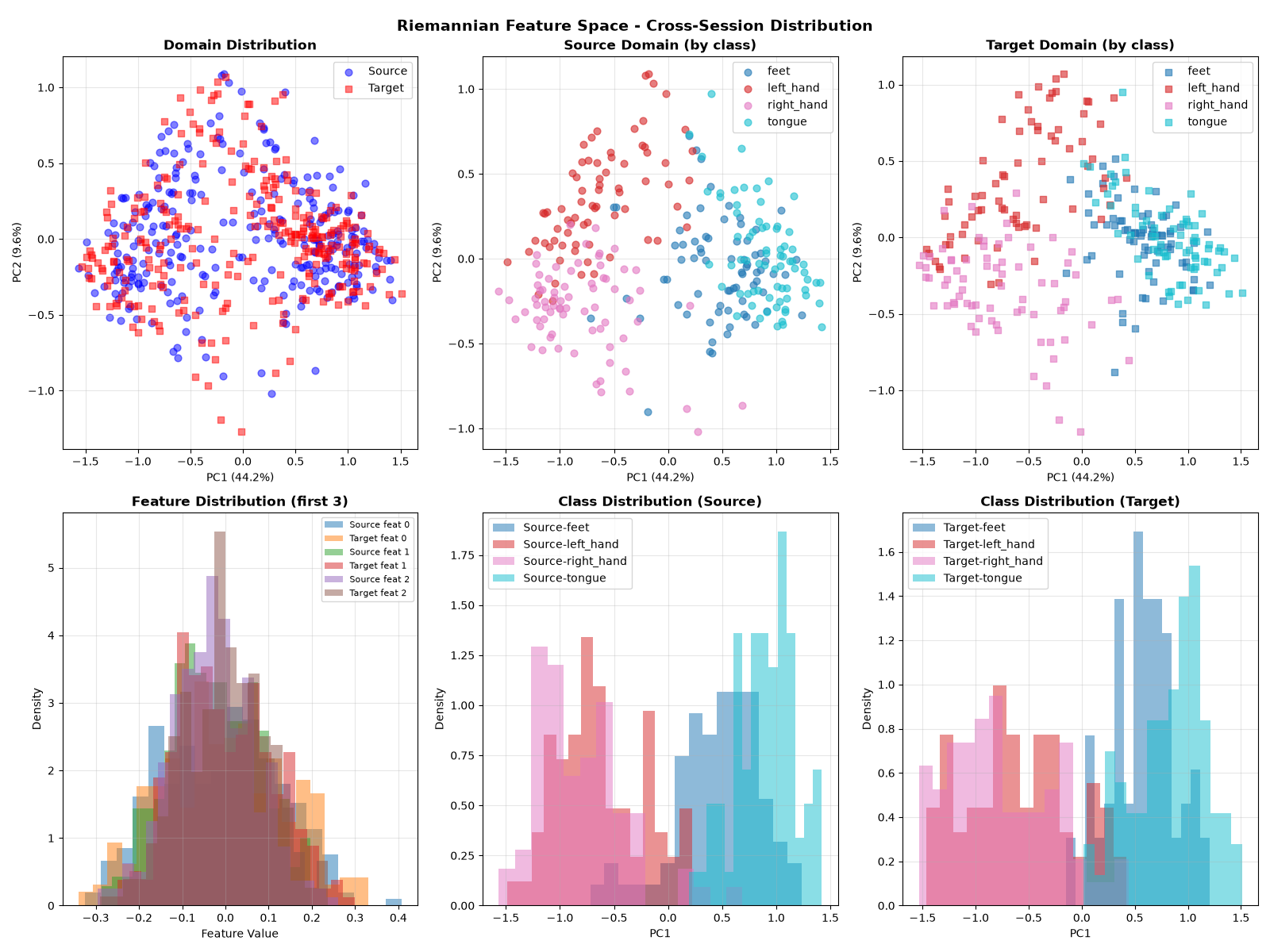
Before applying domain adaptation, let’s visualize the distribution shift between source and target sessions using PCA projection.
class_names = [str(c) for c in le.classes_]
fig = plot_domain_shift_comprehensive(
    features_source,
    features_target,
    y_source,
    y_target,
    class_names=class_names,
    title="Riemannian Feature Space - Cross-Session Distribution",
)
plt.show()

# Prepare data in SKADA format
# SKADA uses sample_domain to distinguish domains:
# - Positive values (1): Source domain
# - Negative values (-1): Target domain
X_combined = np.vstack([features_source, features_target])
y_combined = np.concatenate([y_source, -np.ones(len(y_target))])
sample_domain = np.concatenate(
    [np.ones(len(features_source)), -np.ones(len(features_target))]
)

# Initialize results dictionary
results = {
    "No Adaptation": target_acc_no_adapt,
    "SPDBatchNormMeanVar (TTBN)": target_acc_adapted,
}
CORAL (Correlation Alignment)#
CORAL aligns the second-order statistics (covariance) of source and target feature distributions. This is particularly suitable for SPD-derived features since they already capture covariance structure.
print("\n" + "-" * 50)
print("CORAL (Correlation Alignment)")
print("-" * 50)

coral_pipeline = make_da_pipeline(
    StandardScaler(),
    CORALAdapter(reg=1e-3),
    LogisticRegression(max_iter=1000),
)
coral_pipeline.fit(X_combined, y_combined, sample_domain=sample_domain)
y_pred_coral = coral_pipeline.predict(features_target)
coral_acc = accuracy_score(y_target, y_pred_coral)

print(f"CORAL Accuracy: {coral_acc * 100:.2f}%")
print(f"Improvement over baseline: {(coral_acc - target_acc_no_adapt) * 100:+.2f}%")
results["CORAL"] = coral_acc
--------------------------------------------------
CORAL (Correlation Alignment)
--------------------------------------------------
CORAL Accuracy: 77.08%
Improvement over baseline: +3.82%
Subspace Alignment#
Subspace Alignment learns a linear transformation that aligns the principal subspaces of source and target domains.
print("\n" + "-" * 50)
print("Subspace Alignment")
print("-" * 50)

sa_clf = SubspaceAlignment(
    base_estimator=LogisticRegression(max_iter=1000),
    n_components=min(10, features_source.shape[1]),
)
sa_clf.fit(X_combined, y_combined, sample_domain=sample_domain)
y_pred_sa = sa_clf.predict(features_target)
sa_acc = accuracy_score(y_target, y_pred_sa)

print(f"Subspace Alignment Accuracy: {sa_acc * 100:.2f}%")
print(f"Improvement over baseline: {(sa_acc - target_acc_no_adapt) * 100:+.2f}%")
results["Subspace Alignment"] = sa_acc
--------------------------------------------------
Subspace Alignment
--------------------------------------------------
Subspace Alignment Accuracy: 73.96%
Improvement over baseline: +0.69%
Entropic Optimal Transport#
Optimal Transport finds the minimum cost mapping between source and target distributions. Entropic regularization makes the optimization tractable and provides smoother mappings.
print("\n" + "-" * 50)
print("Entropic Optimal Transport")
print("-" * 50)

try:
    ot_clf = EntropicOTMapping(
        base_estimator=LogisticRegression(max_iter=1000),
        reg_e=1.0,
    )
    ot_clf.fit(X_combined, y_combined, sample_domain=sample_domain)
    y_pred_ot = ot_clf.predict(features_target)
    ot_acc = accuracy_score(y_target, y_pred_ot)

    print(f"Entropic OT Accuracy: {ot_acc * 100:.2f}%")
    print(f"Improvement over baseline: {(ot_acc - target_acc_no_adapt) * 100:+.2f}%")
    results["Entropic OT"] = ot_acc
except Exception as e:
    print(f"Entropic OT failed: {e}")
--------------------------------------------------
Entropic Optimal Transport
--------------------------------------------------
Entropic OT Accuracy: 69.79%
Improvement over baseline: -3.47%
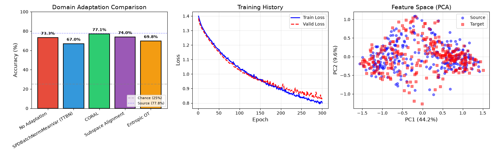
Results Summary#
print("\n" + "=" * 60)
print("Domain Adaptation Results Summary")
print("=" * 60)
print(f"{'Method':<25} {'Accuracy':>12} {'vs Baseline':>14}")
print("-" * 55)
for method, acc in results.items():
    if method == "No Adaptation":
        print(f"{method:<25} {acc * 100:>10.2f}% {'-':>14}")
    else:
        imp = acc - target_acc_no_adapt
        print(f"{method:<25} {acc * 100:>10.2f}% {imp * 100:>+12.2f}%")
print("-" * 55)
print("Chance level: 25.00% (4 classes)")

# Find best method
best_method = max(results.keys(), key=lambda k: results[k])
print(f"\nBest method: {best_method} ({results[best_method] * 100:.2f}%)")
============================================================
Domain Adaptation Results Summary
============================================================
Method                        Accuracy    vs Baseline
-------------------------------------------------------
No Adaptation                  73.26%              -
SPDBatchNormMeanVar (TTBN)      67.01%        -6.25%
CORAL                          77.08%        +3.82%
Subspace Alignment             73.96%        +0.69%
Entropic OT                    69.79%        -3.47%
-------------------------------------------------------
Chance level: 25.00% (4 classes)

Best method: CORAL (77.08%)
Visualizing Results#
fig, axes = plt.subplots(1, 3, figsize=(16, 5))

# 1. Domain Adaptation Methods Comparison
ax1 = axes[0]
methods = list(results.keys())
accuracies = [results[m] * 100 for m in methods]
colors = ["#e74c3c", "#3498db", "#2ecc71", "#9b59b6", "#f39c12"][: len(methods)]
bars = ax1.bar(methods, accuracies, color=colors, edgecolor="black", linewidth=1.5)
ax1.set_ylabel("Accuracy (%)", fontsize=12)
ax1.set_title("Domain Adaptation Comparison", fontsize=14)
ax1.set_ylim([0, 100])
ax1.axhline(y=25, color="gray", linestyle="--", alpha=0.5, label="Chance (25%)")
ax1.axhline(
    y=source_acc * 100,
    color="blue",
    linestyle=":",
    alpha=0.5,
    label=f"Source ({source_acc * 100:.1f}%)",
)

# Add value labels
for bar, acc in zip(bars, accuracies):
    ax1.text(
        bar.get_x() + bar.get_width() / 2,
        bar.get_height() + 2,
        f"{acc:.1f}%",
        ha="center",
        va="bottom",
        fontsize=9,
        fontweight="bold",
    )

ax1.legend(loc="lower right", fontsize=8)
plt.setp(ax1.xaxis.get_majorticklabels(), rotation=30, ha="right")

# 2. Training history
ax2 = axes[1]
history = clf.history
epochs_hist = range(1, len(history) + 1)
ax2.plot(epochs_hist, history[:, "train_loss"], "b-", label="Train Loss", linewidth=2)
ax2.plot(epochs_hist, history[:, "valid_loss"], "r--", label="Valid Loss", linewidth=2)
ax2.set_xlabel("Epoch", fontsize=12)
ax2.set_ylabel("Loss", fontsize=12)
ax2.set_title("Training History", fontsize=14)
ax2.legend(fontsize=10)
ax2.grid(True, alpha=0.3)

# 3. Feature space PCA visualization
ax3 = axes[2]
pca = PCA(n_components=2)
features_all = np.vstack([features_source, features_target])
features_2d = pca.fit_transform(features_all)
n_source = len(features_source)

ax3.scatter(
    features_2d[:n_source, 0],
    features_2d[:n_source, 1],
    c="blue",
    alpha=0.5,
    label="Source",
    marker="o",
    s=30,
)
ax3.scatter(
    features_2d[n_source:, 0],
    features_2d[n_source:, 1],
    c="red",
    alpha=0.5,
    label="Target",
    marker="s",
    s=30,
)
ax3.set_xlabel(f"PC1 ({pca.explained_variance_ratio_[0] * 100:.1f}%)", fontsize=12)
ax3.set_ylabel(f"PC2 ({pca.explained_variance_ratio_[1] * 100:.1f}%)", fontsize=12)
ax3.set_title("Feature Space (PCA)", fontsize=14)
ax3.legend(fontsize=10)
ax3.grid(True, alpha=0.3)

plt.tight_layout()
plt.show()
Understanding SPDBatchNormMeanVar Adaptation#
The key insight is that session variability manifests as a shift in the distribution of SPD matrices. SPDBatchNormMeanVar counters this by:
Centering: Removes the batch mean (Fréchet mean on SPD manifold)
\[\tilde{P}_i = G^{-1/2} P_i G^{-1/2}\]Scaling: Normalizes dispersion
\[\hat{P}_i = \tilde{P}_i^{w/\sqrt{\sigma^2 + \varepsilon}}\]
When we adapt, we update the running mean \(G\) and variance \(\sigma^2\) to match the target domain, aligning the distributions without any labeled data.
Summary#
In this tutorial, we demonstrated:
Training TSMNet on source session
Observing performance drop on target session
Adapting using SPDBatchNormMeanVar (Test-Time Batch Normalization)
Comparing with SKADA domain adaptation methods:
CORAL: Correlation Alignment
Subspace Alignment: Linear subspace mapping
Entropic Optimal Transport: Sample-to-sample mapping
Key insights:
SPDBatchNormMeanVar provides a native Riemannian approach that operates directly on SPD matrices
SKADA methods operate on Euclidean tangent space features and can complement or outperform SPDBatchNormMeanVar depending on the domain shift
Combining multiple approaches allows practitioners to select the best method for their specific use case
Cross-session non-stationarity is a key challenge in BCI. Domain adaptation methods compensate for these shifts by aligning feature distributions between source and target domains.
This unsupervised domain adaptation is particularly valuable in BCI applications where:
Calibration time should be minimized
Users return for multiple sessions
Signal properties drift over time
Total running time of the script: (4 minutes 59.240 seconds)
