Note

Go to the end to download the full example code.

Parallel Transport on SPD Manifolds#

This tutorial explains parallel transport, why it matters for domain adaptation, and how different Riemannian metrics affect transport behavior.

What is Parallel Transport?#

In flat Euclidean space, we can move vectors freely - a vector at one point is “the same” as a vector at another point. On curved manifolds like the SPD manifold, this is not true.

Parallel transport moves a tangent vector along a chosen curve while keeping it “as parallel as possible” according to the manifold’s geometry. The definition is inherently path-dependent on curved manifolds; in this tutorial we use the (unique) AIRM geodesic between \(P\) and \(Q\) unless stated otherwise. For textbook definitions and details, see Optimization Algorithms on Matrix Manifolds and An Introduction to Optimization on Smooth Manifolds. [Absil et al., 2008, Boumal, 2023] Mathematically, if \(\gamma(t)\) is a curve on the manifold and \(X(t)\) is a vector field along \(\gamma\), then \(X\) is parallel if:

\[\nabla_{\dot{\gamma}(t)} X = 0\]

where \(\nabla\) is the Levi-Civita connection.

Key properties of parallel transport:

Linear: \(\Gamma(aU + bV) = a\Gamma(U) + b\Gamma(V)\)
Isometry: Preserves inner products \(\langle \Gamma(U), \Gamma(V) \rangle_Q = \langle U, V \rangle_P\)
Invertible (same curve): Transport \(P \to Q \to P\) recovers the original vector

Setup and Imports #

import matplotlib.pyplot as plt
import torch

from spd_learn.functional import (
    airm_distance,
    parallel_transport_airm,
    parallel_transport_lem,
    parallel_transport_log_cholesky,
    pole_ladder,
    schild_ladder,
    transport_tangent_vector,
)


# For reproducibility
torch.manual_seed(42)


def make_spd(n: int, batch_size: int | None = None) -> torch.Tensor:
    """Create a random SPD matrix."""
    if batch_size is None:
        A = torch.randn(n, n)
    else:
        A = torch.randn(batch_size, n, n)
    eye = torch.eye(n, device=A.device, dtype=A.dtype)
    return A @ A.transpose(-2, -1) + eye


def make_symmetric(n: int, batch_size: int | None = None) -> torch.Tensor:
    """Create a random symmetric matrix (tangent vector)."""
    if batch_size is None:
        V = torch.randn(n, n)
    else:
        V = torch.randn(batch_size, n, n)
    return (V + V.transpose(-2, -1)) / 2

Geometric Intuition #

To understand parallel transport, imagine a tangent vector as an arrow attached to a point on a curved surface. As you slide the base of the arrow along a path, the arrow rotates to stay “parallel” to itself relative to the surface’s curvature.

Tangent space at P          Tangent space at Q
┌─────────────────┐         ┌─────────────────┐
│      V          │         │      Γ(V)       │
│     ↗           │  ───►   │       ↗         │
│    P            │ transport│      Q          │
└─────────────────┘         └─────────────────┘
         │                          │
         └──────────────────────────┘
               SPD Manifold
              (curved space)

Key insight: On flat spaces (Euclidean), vectors don’t change during transport. On curved manifolds like SPD with AIRM, the vector rotates as it moves. LEM and Log-Cholesky flatten the manifold via coordinate maps, so transport is trivial in those coordinates — but non-trivial when expressed in the ambient SPD tangent space.

AIRM Parallel Transport #

Under the Affine-Invariant Riemannian Metric (AIRM), parallel transport along the AIRM geodesic has a closed-form solution. [Bhatia, 2007, Pennec et al., 2006]

\[\Gamma_{P \to Q}(V) = E V E^T\]

where \(E = (QP^{-1})^{1/2}\) is the principal square root of \(QP^{-1}\).

Since \(QP^{-1}\) is generally non-symmetric, SPD Learn computes \(E\) using a numerically stable equivalent formula that only involves symmetric matrix square roots. [Pennec et al., 2006]

\[E = Q^{1/2} (Q^{-1/2} P Q^{-1/2})^{-1/2} Q^{-1/2}\]

This uses only symmetric matrix square roots, which are well-defined and numerically stable for SPD matrices.

# Create two SPD matrices (source and target points)
n = 3
P = make_spd(n)
Q = make_spd(n)

# Create a tangent vector at P
V0 = make_symmetric(n)

# Transport V from T_P to T_Q along the AIRM geodesic
V_transported = parallel_transport_airm(V0, P, Q)

print("Source point P:")
print(P)
print("\nTarget point Q:")
print(Q)
print("\nOriginal tangent vector V at P:")
print(V0)
print("\nTransported tangent vector at Q:")
print(V_transported)

Source point P:
tensor([[ 1.1849, -0.1108,  0.7695],
        [-0.1108,  2.3486,  1.1390],
        [ 0.7695,  1.1390,  6.4963]])

Target point Q:
tensor([[ 2.0127, -1.4075,  1.6247],
        [-1.4075,  6.0662, -1.9787],
        [ 1.6247, -1.9787,  4.3336]])

Original tangent vector V at P:
tensor([[-0.7658, -0.0322,  0.8170],
        [-0.0322, -0.3278,  0.4256],
        [ 0.8170,  0.4256,  0.5227]])

Transported tangent vector at Q:
tensor([[-1.0309, -0.1134,  0.4115],
        [-0.1134, -1.2435,  0.5916],
        [ 0.4115,  0.5916,  0.3206]])

Inner Product Preservation (Isometry)#

The AIRM inner product on tangent vectors is: [Pennec et al., 2006]

\[\langle U, V \rangle_P = \text{tr}(P^{-1} U P^{-1} V)\]

Parallel transport preserves this inner product: \(\langle \Gamma(U), \Gamma(V) \rangle_Q = \langle U, V \rangle_P\)

def airm_inner_product(U, V, P):
    """Compute the AIRM inner product at P (stable solve for SPD matrices)."""
    chol = torch.linalg.cholesky(P)
    p_inv_u = torch.cholesky_solve(U, chol)
    p_inv_v = torch.cholesky_solve(V, chol)
    return torch.trace(p_inv_u @ p_inv_v)


# Create two tangent vectors
U = make_symmetric(n)
V_second = make_symmetric(n)

# Transport both vectors
U_transported = parallel_transport_airm(U, P, Q)
V_second_transported = parallel_transport_airm(V_second, P, Q)

# Compute inner products before and after transport
inner_before = airm_inner_product(U, V_second, P)
inner_after = airm_inner_product(U_transported, V_second_transported, Q)

print(f"Inner product at P: {inner_before:.6f}")
print(f"Inner product at Q: {inner_after:.6f}")
print(f"Difference: {abs(inner_before - inner_after):.2e}")

Inner product at P: -0.294583
Inner product at Q: -0.294583
Difference: 2.68e-07

Roundtrip Consistency #

Transport \(P \to Q \to P\) along the same geodesic (reversed) should recover the original vector. This is a fundamental property of parallel transport along a fixed curve. [Absil et al., 2008]

# Transport V0 from P to Q
V_at_Q = parallel_transport_airm(V0, P, Q)

# Transport back from Q to P
V_recovered = parallel_transport_airm(V_at_Q, Q, P)

# Check that we recovered the original vector
print("Original V:")
print(V0)
print("\nRecovered V after roundtrip:")
print(V_recovered)
print(f"\nReconstruction error: {torch.norm(V0 - V_recovered):.2e}")

Original V:
tensor([[-0.7658, -0.0322,  0.8170],
        [-0.0322, -0.3278,  0.4256],
        [ 0.8170,  0.4256,  0.5227]])

Recovered V after roundtrip:
tensor([[-0.7658, -0.0322,  0.8170],
        [-0.0322, -0.3278,  0.4256],
        [ 0.8170,  0.4256,  0.5227]])

Reconstruction error: 2.79e-06

LEM and Log-Cholesky: Non-trivial Ambient Transport #

Under the Log-Euclidean Metric (LEM), the SPD manifold becomes flat via the matrix logarithm diffeomorphism. Transport is trivial in the log-domain, but when we work with tangent vectors in the ambient SPD space (symmetric matrices), the coordinate change introduces a non-trivial map. [Arsigny et al., 2007, Thanwerdas and Pennec, 2023]

The LEM transport formula is:

\[\Gamma_{P \to Q}^{LEM}(V) = D\exp(\log Q)\bigl[D\log(P)[V]\bigr]\]

where \(D\log(P)\) and \(D\exp(\log Q)\) are Fréchet derivatives. This maps the tangent vector into the flat log-space (where transport is identity), then maps back to the ambient tangent space at Q.

Similarly, the Log-Cholesky metric uses the Cholesky decomposition and log-diagonal map to create flat coordinates. [Lin, 2019] Transport is identity in those coordinates, but the pullback/pushforward through the Cholesky factorization makes it non-trivial in the ambient space.

# All three metrics give non-trivial transport for P != Q
V_lem = parallel_transport_lem(V0, P, Q)
V_chol = parallel_transport_log_cholesky(V0, P, Q)
V_airm = parallel_transport_airm(V0, P, Q)

print("Transport results (all non-trivial for P != Q):")
print(f"  AIRM  - change from V: {torch.norm(V0 - V_airm):.4f}")
print(f"  LEM   - change from V: {torch.norm(V0 - V_lem):.4f}")
print(f"  L-Chol - change from V: {torch.norm(V0 - V_chol):.4f}")

# Self-transport (P -> P) should be identity for all metrics
V_lem_self = parallel_transport_lem(V0, P, P)
V_chol_self = parallel_transport_log_cholesky(V0, P, P)
print("\nSelf-transport (P -> P) is identity:")
print(f"  LEM:        {torch.allclose(V0, V_lem_self, atol=1e-5)}")
print(f"  Log-Cholesky: {torch.allclose(V0, V_chol_self, atol=1e-5)}")

Transport results (all non-trivial for P != Q):
  AIRM  - change from V: 1.1605
  LEM   - change from V: 1.1181
  L-Chol - change from V: 1.1831

Self-transport (P -> P) is identity:
  LEM:        True
  Log-Cholesky: True

Comparing Transport Methods #

SPD Learn provides several transport methods with different trade-offs:

Method	Formula	Complexity	Notes
AIRM	\(EVE^T\)	O(n³)	Exact, preserves geometry
LEM	Fréchet derivatives	O(n³)	Via D_exp(log Q)[D_log(P)]
Log-Cholesky	Cholesky pull/push	O(n³)	Via log-diagonal map
Schild’s ladder	Iterative	O(k·n³)	~O(1/k²) (small steps)
Pole ladder	Single iteration	O(n³)	O(h²) (small distance)

The transport_tangent_vector function provides a unified interface:

# Transport using different metrics
V_airm = transport_tangent_vector(V0, P, Q, metric="airm")
V_lem = transport_tangent_vector(V0, P, Q, metric="lem")
V_chol = transport_tangent_vector(V0, P, Q, metric="log_cholesky")

print("Transport results by metric (all differ from each other):")
print(f"  AIRM vs LEM difference:          {torch.norm(V_airm - V_lem):.4f}")
print(f"  AIRM vs Log-Cholesky difference: {torch.norm(V_airm - V_chol):.4f}")
print(f"  LEM vs Log-Cholesky difference:  {torch.norm(V_lem - V_chol):.4f}")

Transport results by metric (all differ from each other):
  AIRM vs LEM difference:          0.1865
  AIRM vs Log-Cholesky difference: 1.6314
  LEM vs Log-Cholesky difference:  1.6406

Numerical Approximations: Schild’s and Pole Ladder #

When closed-form transport is unavailable, numerical methods approximate transport using geodesics:

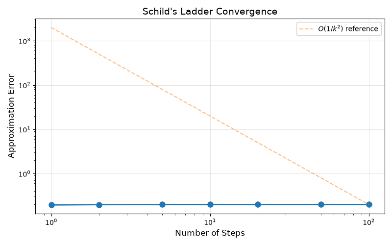
Schild’s Ladder: Iterative parallelogram construction along the geodesic. Each step uses geodesic midpoints to approximate parallel translation. For sufficiently small step sizes, the approximation error scales like O(1/k²) in the number of steps. [Lorenzi and Pennec, 2014]

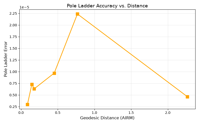
Pole Ladder: A more efficient variant using a single reflection through the geodesic midpoint. For small geodesic distances, the local error is O(h²) where h is the distance between P and Q. [Lorenzi and Pennec, 2014]

# Compare Schild's ladder with different step counts
V_schild_5 = schild_ladder(V0, P, Q, n_steps=5)
V_schild_10 = schild_ladder(V0, P, Q, n_steps=10)
V_schild_20 = schild_ladder(V0, P, Q, n_steps=20)

# Pole ladder (single step)
V_pole = pole_ladder(V0, P, Q)

# Compare to exact AIRM transport
V_exact = parallel_transport_airm(V0, P, Q)

print("Approximation errors (compared to exact AIRM):")
print(f"  Schild's ladder (5 steps):  {torch.norm(V_exact - V_schild_5):.6f}")
print(f"  Schild's ladder (10 steps): {torch.norm(V_exact - V_schild_10):.6f}")
print(f"  Schild's ladder (20 steps): {torch.norm(V_exact - V_schild_20):.6f}")
print(f"  Pole ladder:                {torch.norm(V_exact - V_pole):.6f}")

Approximation errors (compared to exact AIRM):
  Schild's ladder (5 steps):  0.198965
  Schild's ladder (10 steps): 0.199101
  Schild's ladder (20 steps): 0.199139
  Pole ladder:                0.000021

Visualizing Convergence of Schild’s Ladder #

Let’s see how Schild’s ladder converges to the exact solution as we increase the number of steps.

steps = [1, 2, 5, 10, 20, 50, 100]
errors = []

for n_steps in steps:
    V_approx = schild_ladder(V0, P, Q, n_steps=n_steps)
    error = torch.norm(V_exact - V_approx).item()
    errors.append(error)

plt.figure(figsize=(8, 5))
plt.loglog(steps, errors, "o-", linewidth=2, markersize=8)
plt.xlabel("Number of Steps", fontsize=12)
plt.ylabel("Approximation Error", fontsize=12)
plt.title("Schild's Ladder Convergence", fontsize=14)
plt.grid(True, alpha=0.3)

# Add reference line for O(1/k²) convergence (anchored at the largest k)
reference = [errors[-1] * (steps[-1] / s) ** 2 for s in steps]
plt.loglog(steps, reference, "--", alpha=0.5, label=r"$O(1/k^2)$ reference")
plt.legend()
plt.tight_layout()
plt.show()

Pole Ladder Error vs. Geodesic Distance #

Pole ladder’s error depends on the geodesic distance between P and Q. For nearby points, it’s very accurate; for distant points, error grows.

distances = []
pole_errors = []

# Generate pairs with varying distances
for scale in [0.1, 0.3, 0.5, 1.0, 2.0, 3.0]:
    P_test = make_spd(n)
    # Create Q at controlled distance from P
    direction = make_symmetric(n)
    direction = direction / torch.norm(direction) * scale
    Q_test = P_test @ torch.linalg.matrix_exp(torch.linalg.solve(P_test, direction))

    V_test = make_symmetric(n)
    V_exact_test = parallel_transport_airm(V_test, P_test, Q_test)
    V_pole_test = pole_ladder(V_test, P_test, Q_test)

    dist = airm_distance(P_test, Q_test).item()
    err = torch.norm(V_exact_test - V_pole_test).item()
    distances.append(dist)
    pole_errors.append(err)

plt.figure(figsize=(8, 5))
plt.plot(distances, pole_errors, "s-", linewidth=2, markersize=8, color="orange")
plt.xlabel("Geodesic Distance (AIRM)", fontsize=12)
plt.ylabel("Pole Ladder Error", fontsize=12)
plt.title("Pole Ladder Accuracy vs. Distance", fontsize=14)
plt.grid(True, alpha=0.3)
plt.tight_layout()
plt.show()

print("Pole ladder error increases with geodesic distance.")
print("Use Schild's ladder (more steps) for distant points.")

Pole ladder error increases with geodesic distance.
Use Schild's ladder (more steps) for distant points.

Timing Comparison #

Different transport methods have different computational costs. Here we compare wall-clock time for a realistic matrix size.

import time


n_timing = 22  # Typical EEG channel count
n_trials = 50

P_time = make_spd(n_timing)
Q_time = make_spd(n_timing)
V_time = make_symmetric(n_timing)


def benchmark(func, *args, n_runs=n_trials):
    """Benchmark a function and return mean time in milliseconds."""
    # Warmup
    for _ in range(3):
        func(*args)
    # Timed runs
    start = time.perf_counter()
    for _ in range(n_runs):
        func(*args)
    elapsed = time.perf_counter() - start
    return (elapsed / n_runs) * 1000  # Convert to ms


time_airm = benchmark(parallel_transport_airm, V_time, P_time, Q_time)
time_lem = benchmark(parallel_transport_lem, V_time, P_time, Q_time)
time_schild_10 = benchmark(schild_ladder, V_time, P_time, Q_time, n_trials)
time_pole = benchmark(pole_ladder, V_time, P_time, Q_time)

print(f"\nTiming comparison ({n_timing}x{n_timing} matrices, {n_trials} runs):")
print(f"  AIRM (congruence):    {time_airm:.3f} ms")
print(f"  LEM (Frechet derivs): {time_lem:.3f} ms")
print(f"  Schild's (10 steps):  {time_schild_10:.3f} ms")
print(f"  Pole ladder:          {time_pole:.3f} ms")

Timing comparison (22x22 matrices, 50 runs):
  AIRM (congruence):    0.511 ms
  LEM (Frechet derivs): 0.488 ms
  Schild's (10 steps):  79.890 ms
  Pole ladder:          1.201 ms

Application: Cross-Subject EEG Transfer #

In Brain-Computer Interface (BCI) applications, different subjects have different “reference” covariance matrices due to anatomical and physiological differences. Parallel transport enables aligning tangent vectors from different subjects to a common reference, which is essential for cross-subject transfer learning.

Scenario: Subject A has labeled training data, Subject B has no labels. We want to use Subject A’s classifier on Subject B’s data.

Parallel Transport vs. Batch Normalization #

Both parallel transport and SPD batch normalization address distribution shift, but they work differently:

Parallel transport: Moves tangent vectors between reference points on the manifold. Use when combining tangent vectors from different reference points.
SPDBatchNormMeanVar: Normalizes SPD matrices to a common scale by centering around the geometric mean and scaling the variance. Use when aligning statistical properties of SPD matrices directly.

The choice depends on your pipeline:

If you work in tangent space: use parallel transport
If you work with SPD matrices directly: use batch normalization

Choosing the Right Method #

Here’s a decision guide for selecting the appropriate transport method:

Need affine invariance? → Use AIRM transport
Need consistency with pyRiemann? → LEM and Log-Cholesky now match pyRiemann’s non-trivial transport conventions
No closed-form available? → Use pole ladder for small distances
High accuracy needed? → Use Schild’s ladder with many steps
Need gradients through reference points? → All three closed-form methods (AIRM, LEM, Log-Cholesky) support autograd

# Gradient flow demonstration
P_grad = make_spd(n)
Q_grad = make_spd(n)
V_grad = make_symmetric(n)

P_grad.requires_grad_(True)
Q_grad.requires_grad_(True)
V_grad.requires_grad_(True)

# Transport with gradient tracking
V_out = parallel_transport_airm(V_grad, P_grad, Q_grad)
loss = V_out.sum()
loss.backward()

print("Gradient flow through parallel transport:")
print(f"  grad_V exists: {V_grad.grad is not None}")
print(f"  grad_P exists: {P_grad.grad is not None}")
print(f"  grad_Q exists: {Q_grad.grad is not None}")

Gradient flow through parallel transport:
  grad_V exists: True
  grad_P exists: True
  grad_Q exists: True

Common Pitfalls and Numerical Stability #

Parallel transport can encounter numerical issues in certain scenarios. Here’s how to handle them:

1. Ill-conditioned matrices (near-singular)

When P or Q have very small eigenvalues, matrix inversions become unstable.

# Example: ill-conditioned matrix
P_illcond = torch.diag(torch.tensor([1.0, 1.0, 1e-8]))
Q_good = make_spd(3)
V_test = make_symmetric(3)

# Check condition number
cond_P = torch.linalg.cond(P_illcond).item()
print("\nNumerical stability example:")
print(f"  Condition number of P: {cond_P:.2e}")
print("  (Values > 1e10 may cause issues)")

# Solution: regularize by adding small diagonal
epsilon = 1e-6
P_regularized = P_illcond + epsilon * torch.eye(3)
cond_reg = torch.linalg.cond(P_regularized).item()
print(f"  After regularization: {cond_reg:.2e}")

Numerical stability example:
  Condition number of P: 1.00e+08
  (Values > 1e10 may cause issues)
  After regularization: 9.90e+05

2. Large geodesic distances

When P and Q are very far apart on the manifold, numerical errors accumulate. Use higher precision (float64) or Schild’s ladder with more steps.

P_f64 = make_spd(n).double()
Q_f64 = make_spd(n).double()
V_f64 = make_symmetric(n).double()

V_transported_f64 = parallel_transport_airm(V_f64, P_f64, Q_f64)
print("\nUsing float64 for better precision:")
print(f"  Input dtype: {V_f64.dtype}")
print(f"  Output dtype: {V_transported_f64.dtype}")

Using float64 for better precision:
  Input dtype: torch.float64
  Output dtype: torch.float64

3. Asymmetry in transported vectors

Due to floating-point errors, transported vectors may become slightly asymmetric. Re-symmetrize if needed for downstream operations.

V_transported_check = parallel_transport_airm(V0, P, Q)
asymmetry = torch.norm(V_transported_check - V_transported_check.T).item()
print("\nAsymmetry check:")
print(f"  Asymmetry norm: {asymmetry:.2e}")

# Re-symmetrize if needed
V_resym = (V_transported_check + V_transported_check.T) / 2
print(f"  After re-symmetrization: {torch.norm(V_resym - V_resym.T):.2e}")

Asymmetry check:
  Asymmetry norm: 1.21e-07
  After re-symmetrization: 0.00e+00

Summary #

In this tutorial, we covered:

Parallel transport moves tangent vectors while preserving geometry
AIRM uses the congruence formula \(EVE^T\)
LEM uses Fréchet derivatives of matrix log/exp [Thanwerdas and Pennec, 2023]
Log-Cholesky uses Cholesky pullback/pushforward [Lin, 2019]
All three are non-trivial in the ambient SPD tangent space (flat geometry only applies in their respective coordinate systems)
Numerical methods (Schild’s and pole ladder) approximate transport when closed-form solutions are unavailable or expensive
Cross-subject transfer is a key application for BCI domain adaptation