spd_learn.modules.WaveletConv

class spd_learn.modules.WaveletConv(kernel_width_s: float, foi_init: Sequence[float] | Tensor, sfreq: int = 100, fwhm_init: Sequence[float] | Tensor | None = None, padding: int | str = 0, stride: int = 1, scaling: str = 'oct', dtype: dtype = torch.complex64, device: device | None = None)

Bases: Module

Parametrized Complex Gabor Wavelet Convolution Layer.

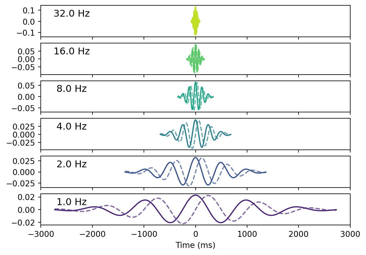
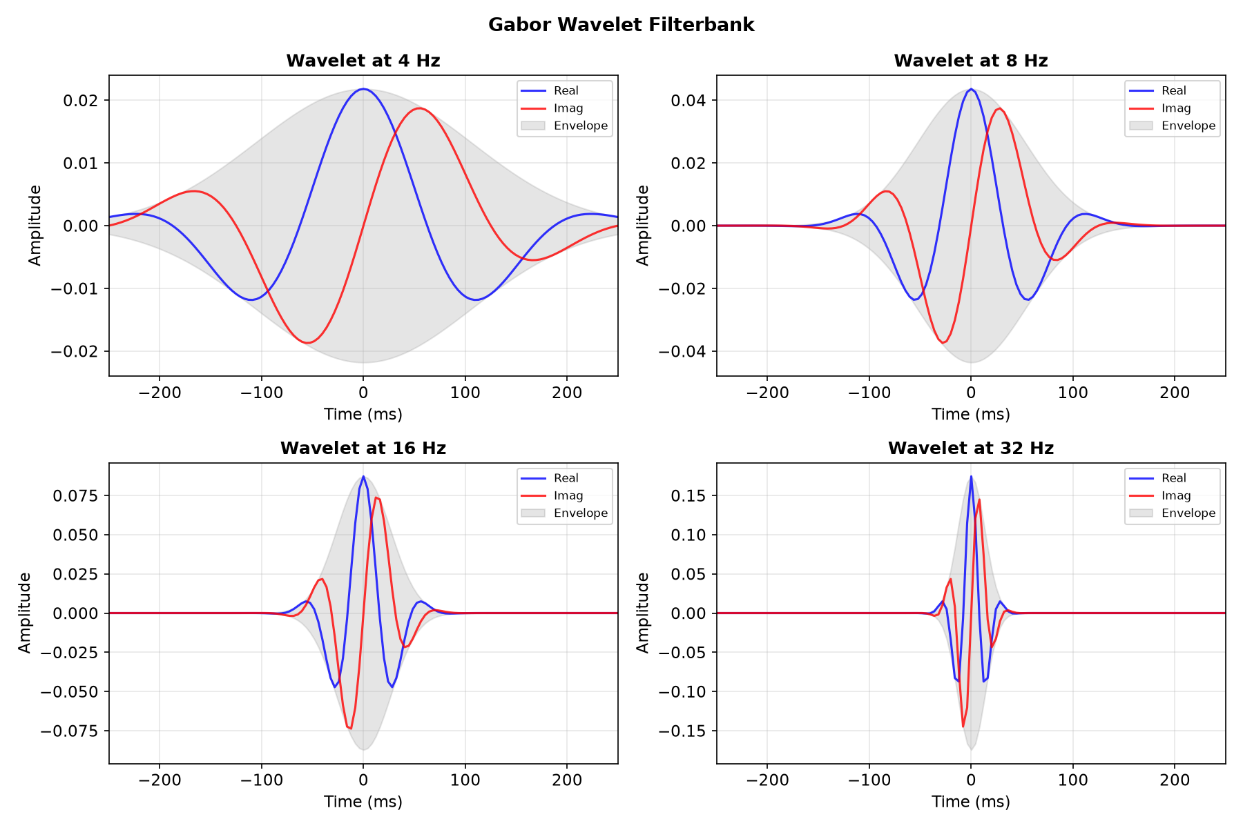
This layer performs a 1D convolution of input signals with a bank of complex-valued Gabor wavelets (Morlet wavelets). The center frequency and temporal resolution of each wavelet are learnable parameters.

Parameters:

• kernel_width_s (float) – The temporal width of the wavelet kernel in seconds.

• foi_init (Sequence[float]) – A sequence of initial center frequencies for the wavelets, in octaves.

• sfreq (int, default=100) – The sampling frequency of the input data in Hz.

• fwhm_init (Sequence[float], optional) – A sequence of initial Full Width at Half Maximums (FWHM) for the wavelets, in octaves.

• padding (int or str, default=0) – Padding mode for the convolution.

• stride (int, default=1) – The stride of the convolution.

• scaling (str, default="oct") – The scaling method applied to the wavelets after L2 normalization.

• dtype (torch.dtype, default=torch.complex64) – The data type for the complex wavelet kernels.

Notes

See [Paillard et al., 2025] for more details.

Examples

>>> import torch
>>> from spd_learn.modules import WaveletConv
>>> # Create wavelet layer with 5 wavelets centered at 4, 8, 16, 32, 64 Hz
>>> foi_init = [2.0, 3.0, 4.0, 5.0, 6.0]  # In octaves (2^n Hz)
>>> wavelet = WaveletConv(kernel_width_s=0.5, foi_init=foi_init, sfreq=250)
>>> X = torch.randn(2, 22, 500)  # (batch, channels, time)
>>> Y = wavelet(X)
>>> Y.shape
torch.Size([2, 5, 22, 376])

import torch
import numpy as np
import matplotlib.pyplot as plt
from spd_learn.modules import WaveletConv
from spd_learn.functional import compute_gabor_wavelet

# Create wavelet filterbank
foi_init = [2.0, 3.0, 4.0, 5.0]  # 4, 8, 16, 32 Hz
sfreq = 250
wavelet = WaveletConv(kernel_width_s=0.5, foi_init=foi_init, sfreq=sfreq)

# Get wavelet kernels
tt = wavelet.tt.numpy()
wavelets = compute_gabor_wavelet(
    wavelet.tt, wavelet.foi, wavelet.fwhm, sfreq=sfreq
).detach().numpy()

fig, axes = plt.subplots(2, 2, figsize=(12, 8))

freq_labels = [f'{2**f:.0f} Hz' for f in foi_init]

for i, (ax, wav, label) in enumerate(zip(axes.flat, wavelets, freq_labels)):
    ax.plot(tt * 1000, wav.real, 'b-', label='Real', alpha=0.8)
    ax.plot(tt * 1000, wav.imag, 'r-', label='Imag', alpha=0.8)
    ax.fill_between(tt * 1000, -np.abs(wav), np.abs(wav),
                    color='gray', alpha=0.2, label='Envelope')
    ax.set_xlabel('Time (ms)')
    ax.set_ylabel('Amplitude')
    ax.set_title(f'Wavelet at {label}', fontweight='bold')
    ax.legend(fontsize=8)
    ax.grid(True, alpha=0.3)
    ax.set_xlim(tt[0]*1000, tt[-1]*1000)

plt.suptitle('Gabor Wavelet Filterbank', fontsize=13, fontweight='bold')
plt.tight_layout()
plt.show()

(Source code)

forward(X: Tensor) → Tensor

Applies the wavelet convolution to the input signal.

Parameters:

X (torch.Tensor) – Input data tensor with shape (N, C_in, T_in) or (N, E, C_in, T_in).

Returns:

Complex-valued output tensor after convolution.

Return type:

torch.Tensor

tt: Tensor