spd_learn.modules.CovLayer

class spd_learn.modules.CovLayer(method: Callable = <function covariance>, device=None, dtype=None)

Bases: Module

Covariance Estimation Layer for Neuroimaging Data.

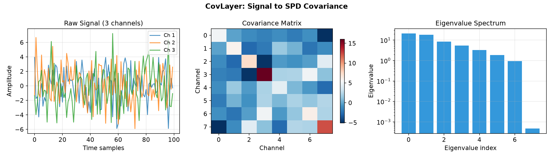
This layer computes spatial covariance matrices from multivariate time series, transforming input data of shape (…, n_channels, n_times) into SPD matrices of shape (…, n_channels, n_channels).

Mathematical Definition

Given a data segment \(X \in \mathbb{R}^{n_C \times n_T}\) formed by concatenating \(n_T\) consecutive time samples:

\[X = [x(t), x(t+1), \ldots, x(t+n_T-1)]\]

The spatial covariance matrix is defined as the second-order moment:

\[C = \mathbb{E}[x(t) x(t)^\top] \in \mathcal{S}_{+}^{n_C}\]

capturing linear statistical dependencies across spatial channels. In practice, this is estimated as \(\hat{C} = \frac{1}{n_T-1} X X^\top\) after centering.

Statistical Assumptions

The covariance estimator assumes approximate stationarity within the temporal window. The true covariance is strictly positive definite if the underlying process is nondegenerate; however, empirical estimates may be:

• Rank-deficient when \(n_T < n_C\) (more channels than time samples)

• Ill-conditioned due to strong linear dependencies or narrow-band filtering

For ill-conditioned cases, consider using Shrinkage regularization.

Neuroimaging Context

• EEG/MEG/ECoG: Spatial covariance summarizes pairwise dependencies between neural signals, encoding task-relevant spectral modulations (ERD/ERS).

• fMRI: Applied to parcellated regional time series to compute functional connectivity matrices.

Parameters:

• method (Callable, default=covariance) –

  The covariance estimation method. Options:

  • covariance: Standard empirical covariance

  • sample_covariance: With Bessel correction (divides by n-1)

  • real_covariance: For complex-valued signals

  • cross_covariance: Cross-covariance between channel groups

• device (torch.device, optional) – The device to move the covariance matrices to.

• dtype (torch.dtype, optional) – The data type to cast the covariance matrices to.

See also

Shrinkage

Regularizes ill-conditioned covariance matrices.

BiMap

Bilinear mapping for covariance dimensionality reduction.

SPDBatchNormMeanVar

Batch normalization on the SPD manifold.

Examples

>>> import torch
>>> from spd_learn.modules import CovLayer
>>> x = torch.randn(10, 20, 100)
>>> cov_layer = CovLayer()
>>> cov = cov_layer(x)
>>> cov.shape
torch.Size([10, 20, 20])

import torch
import numpy as np
import matplotlib.pyplot as plt
from spd_learn.modules import CovLayer

# Generate synthetic multivariate time series
torch.manual_seed(42)
batch_size, n_channels, n_times = 1, 8, 100

# Create correlated signals
raw_signals = torch.randn(batch_size, n_channels, n_times)
mixing = torch.randn(n_channels, n_channels)
raw_signals = torch.einsum('ij,bjt->bit', mixing, raw_signals)

# Apply CovLayer
cov_layer = CovLayer()
covariances = cov_layer(raw_signals)

fig, axes = plt.subplots(1, 3, figsize=(14, 4))

# Raw signal
ax1 = axes[0]
for i in range(3):
    ax1.plot(raw_signals[0, i, :].numpy(), label=f'Ch {i+1}', alpha=0.8)
ax1.set_xlabel('Time samples')
ax1.set_ylabel('Amplitude')
ax1.set_title('Raw Signal (3 channels)')
ax1.legend(fontsize=9)
ax1.grid(True, alpha=0.3)

# Covariance matrix
ax2 = axes[1]
im = ax2.imshow(covariances[0].numpy(), cmap='RdBu_r', aspect='auto')
ax2.set_title('Covariance Matrix')
ax2.set_xlabel('Channel')
ax2.set_ylabel('Channel')
plt.colorbar(im, ax=ax2, shrink=0.8)

# Eigenvalue spectrum
ax3 = axes[2]
eigvals = torch.linalg.eigvalsh(covariances[0]).numpy()
ax3.bar(range(n_channels), sorted(eigvals, reverse=True), color='#3498db')
ax3.set_xlabel('Eigenvalue index')
ax3.set_ylabel('Eigenvalue')
ax3.set_title('Eigenvalue Spectrum')
ax3.set_yscale('log')
ax3.grid(True, alpha=0.3)

plt.suptitle('CovLayer: Signal to SPD Covariance', fontweight='bold')
plt.tight_layout()
plt.show()

(Source code)

forward(x: Tensor) → Tensor

Forward pass.

Parameters:

x (torch.Tensor) – Input data of shape (…, n_channels, n_times).

Returns:

Covariance matrices of shape (…, n_channels, n_channels).

Return type:

torch.Tensor