spd_learn.modules.TraceNorm

class spd_learn.modules.TraceNorm(epsilon: float = 0.0, device=None, dtype=None)

Bases: Module

Trace Normalization Layer for Scale-Invariant Covariance.

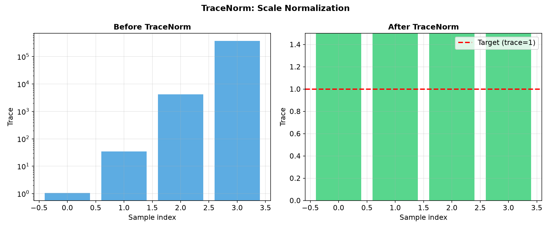
This module normalizes each covariance matrix by its trace, producing matrices with unit trace, and adds a small diagonal regularization:

\[X_{\text{out}} = \frac{X}{\text{tr}(X)} + \epsilon I\]

Geometric Interpretation

Trace normalization removes scale information while preserving the correlation structure of the covariance matrix. This is particularly useful when comparing covariances across subjects or sessions with different overall signal amplitudes.

For SPD matrices, this operation maps to a lower-dimensional submanifold of unit-trace SPD matrices, which can simplify geometric computations while retaining the relative eigenvalue structure.

Parameters:

epsilon (float, default=0.0) – A small value added to the diagonal for numerical stability. Ensures positive definiteness when trace normalization produces near-singular matrices.

See also

Shrinkage

Regularization via shrinkage toward identity.

Examples

>>> import torch
>>> from spd_learn.modules import TraceNorm
>>> trace_norm = TraceNorm(epsilon=1e-5)
>>> X = torch.randn(4, 8, 8)
>>> X = X @ X.mT  # Make SPD
>>> Y = trace_norm(X)
>>> Y.shape
torch.Size([4, 8, 8])

import torch
import numpy as np
import matplotlib.pyplot as plt
from spd_learn.modules import TraceNorm, CovLayer

torch.manual_seed(42)

# Generate synthetic data with different scales
n_channels = 6
batch_size = 4

# Create covariances with varying scales
covariances = []
for scale in [0.1, 1.0, 10.0, 100.0]:
    A = torch.randn(n_channels, n_channels) * scale
    cov = A @ A.T + 0.1 * torch.eye(n_channels)
    covariances.append(cov)
covariances = torch.stack(covariances)

# Apply TraceNorm
trace_norm = TraceNorm(epsilon=1e-5)
normalized = trace_norm(covariances)

fig, axes = plt.subplots(1, 2, figsize=(12, 5))

# Before normalization - traces vary widely
ax1 = axes[0]
traces_before = [torch.trace(covariances[i]).item() for i in range(batch_size)]
ax1.bar(range(batch_size), traces_before, color='#3498db', alpha=0.8)
ax1.set_xlabel('Sample index')
ax1.set_ylabel('Trace')
ax1.set_title('Before TraceNorm', fontweight='bold')
ax1.set_yscale('log')
ax1.grid(True, alpha=0.3)

# After normalization - traces are ~1
ax2 = axes[1]
traces_after = [torch.trace(normalized[i]).item() for i in range(batch_size)]
ax2.bar(range(batch_size), traces_after, color='#2ecc71', alpha=0.8)
ax2.set_xlabel('Sample index')
ax2.set_ylabel('Trace')
ax2.set_title('After TraceNorm', fontweight='bold')
ax2.axhline(y=1.0, color='red', linestyle='--', linewidth=2, label='Target (trace=1)')
ax2.legend()
ax2.grid(True, alpha=0.3)
ax2.set_ylim(0, 1.5)

plt.suptitle('TraceNorm: Scale Normalization', fontweight='bold')
plt.tight_layout()
plt.show()

(Source code)

forward(covariances: Tensor) → Tensor

Forward pass of the TraceNorm layer.

Parameters:

covariances (torch.Tensor) – A batch of covariance matrices with shape (…, n, n).

Returns:

The trace-normalized covariance matrices.

Return type:

torch.Tensor