spd_learn.modules.Shrinkage

class spd_learn.modules.Shrinkage(n_chans: int, init_shrinkage: float = 0.0, learnable: bool = False, device=None, dtype=None)

Bases: Module

Learnable Shrinkage Regularization for Covariance Matrices.

This module applies a learnable shrinkage transformation inspired by the Ledoit-Wolf and Oracle Approximating Shrinkage (OAS) estimators [Ledoit and Wolf, 2004] to regularize covariance matrices:

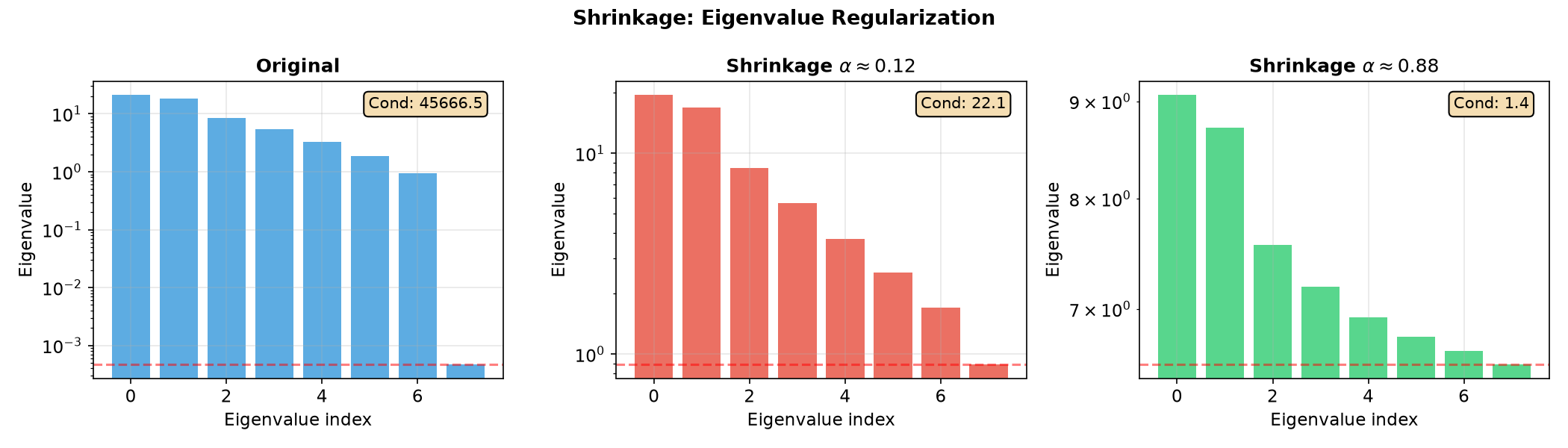
\[\hat{C} = (1 - \alpha) C + \alpha \cdot \frac{\text{tr}(C)}{n} \cdot I_n\]

where \(\alpha \in [0, 1]\) is the shrinkage intensity and \(n\) is the matrix dimension. This convex combination interpolates between the empirical covariance \(C\) and a structured target (scaled identity).

Why Shrinkage is Necessary

Reliable covariance estimation in neuroimaging faces three fundamental challenges [Varoquaux et al., 2010]:

1. Curse of dimensionality: When the number of variables exceeds the number of samples (\(n_C > n_T\)), empirical covariance estimates become ill-conditioned or rank-deficient.

2. Non-Gaussian artifacts: Outliers such as eye blinks in EEG or head motion in fMRI violate distributional assumptions.

3. Temporal non-stationarity: Brain signals evolve over time, breaking i.i.d. assumptions and causing estimation errors to propagate.

Shrinkage estimators address these issues by trading variance for bias, pulling extreme eigenvalues toward a common mean, which improves conditioning and stability of downstream analyses. Automated model selection methods can determine the optimal shrinkage estimator for MEG and EEG applications [Engemann and Gramfort, 2015].

Typical Pipeline

Shrinkage is typically the final step in covariance regularization [Aristimunha et al., 2026]:

1. Normalize time series: Zero mean and unit L2 norm per channel

2. Compute sample covariance: \(C = XX^T\)

3. Apply shrinkage: \(\hat{C} = (1-\alpha)C + \alpha \cdot \text{tr}(C)/n \cdot I\)

Limitations

While shrinkage estimators are theoretically well-founded, they rely on structured targets (e.g., scaled identity) that may not capture complex covariance structure in densely connected brain networks. This limitation motivates alternative approaches such as population-level shrinkage [Rahim et al., 2017].

Parameters:

• n_chans (int) – The size of the square matrices expected as input.

• init_shrinkage (float, default=0.0) – The initial value for the pre-sigmoid shrinkage parameter. After sigmoid: 0.0 → α ≈ 0.5, negative → less shrinkage, positive → more.

• learnable (bool, default=False) – If True, the shrinkage parameter is learned during training.

Notes

The optimal shrinkage intensity depends on the sample size, dimensionality, and signal properties. The Ledoit-Wolf estimator provides an analytical formula for the optimal \(\alpha\), while this module allows learning it from data when learnable=True.

See also

TraceNorm

Normalizes by trace without shrinkage.

CovLayer

Computes covariance matrices from time series.

Examples

>>> import torch
>>> from spd_learn.modules import Shrinkage
>>> shrinkage = Shrinkage(n_chans=8, init_shrinkage=0.5, learnable=True)
>>> X = torch.randn(4, 8, 8)
>>> X = X @ X.mT  # Make SPD
>>> Y = shrinkage(X)
>>> Y.shape
torch.Size([4, 8, 8])

import torch
import numpy as np
import matplotlib.pyplot as plt
from spd_learn.modules import Shrinkage, CovLayer

torch.manual_seed(42)

# Generate synthetic data and compute covariance
n_channels = 8
raw_signals = torch.randn(1, n_channels, 100)
mixing = torch.randn(n_channels, n_channels)
raw_signals = torch.einsum('ij,bjt->bit', mixing, raw_signals)

cov_layer = CovLayer()
covariances = cov_layer(raw_signals)

# Apply shrinkage with different coefficients
shrinkage_low = Shrinkage(n_chans=n_channels, init_shrinkage=-2.0)  # ~0.12
shrinkage_high = Shrinkage(n_chans=n_channels, init_shrinkage=2.0)  # ~0.88

cov_low = shrinkage_low(covariances)
cov_high = shrinkage_high(covariances)

fig, axes = plt.subplots(1, 3, figsize=(14, 4))

# Original eigenvalues
eigvals_orig = torch.linalg.eigvalsh(covariances[0]).numpy()
eigvals_low = torch.linalg.eigvalsh(cov_low[0].detach()).numpy()
eigvals_high = torch.linalg.eigvalsh(cov_high[0].detach()).numpy()

for ax, eigv, title, color in zip(
    axes,
    [eigvals_orig, eigvals_low, eigvals_high],
    ['Original', r'Shrinkage $\alpha \approx 0.12$', r'Shrinkage $\alpha \approx 0.88$'],
    ['#3498db', '#e74c3c', '#2ecc71']
):
    ax.bar(range(n_channels), sorted(eigv, reverse=True), color=color, alpha=0.8)
    ax.set_xlabel('Eigenvalue index')
    ax.set_ylabel('Eigenvalue')
    ax.set_title(title, fontweight='bold')
    ax.set_yscale('log')
    ax.grid(True, alpha=0.3)
    ax.axhline(y=min(eigv), color='red', linestyle='--', alpha=0.5)
    cond = max(eigv) / min(eigv)
    ax.text(0.95, 0.95, f'Cond: {cond:.1f}', transform=ax.transAxes,
            ha='right', va='top', fontsize=10, bbox=dict(boxstyle='round', facecolor='wheat'))

plt.suptitle('Shrinkage: Eigenvalue Regularization', fontweight='bold')
plt.tight_layout()
plt.show()

(Source code)

forward(X: Tensor) → Tensor

Forward pass of the Shrinkage layer.

Parameters:

X (torch.Tensor) – Input tensor of shape (…, n_chans, n_chans).

Returns:

The regularized output tensor.

Return type:

torch.Tensor

identity_matrix: Tensor